The AD-AS model
- Details
- Category: Macroeconomics
- Hits: 14,511
The problem with the IS-LM model
The starting point of the Aggregate Demand - Aggregate Supply or AD-AS model is an assumption in the IS-LM model (and in the cross model) that limits its usefulness. This is the assumption that if firms where to choose the profit maximizing quantity of L (LOPT), they would produce more than the aggregate demand. In the IS-LM, YOPT > YD must hold as discussed in section Aggregate supply.
To realize why this is a problem in the IS-LM model, we gradually increase the aggregate demand byincreasing G. We can illustrate the process using figure 12.6 in Section The Labor Market
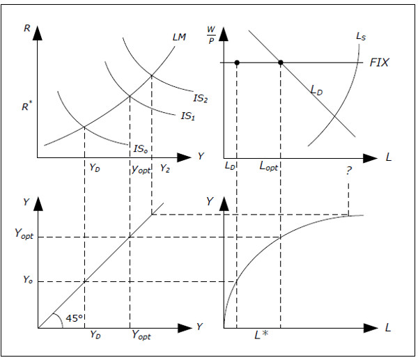
Fig. 13.1: Illustrating the problem in the IS-LM model
- Let us begin with a given real wage W/P, an IS curve (IS0) and an LM curve. In equilibrium, we will have Y = Y0 and L = L0.
- Now increase G so that IS curve shifts outwards from IS0 to IS1. In the first step, we increase G just enough so that Y = YOPT in equilibrium, i.e. exactly to the level that firms want to produce at the given real wage.
- Firms will now want to hire LOPT which is precisely the profit-maximizing quantity of L. It isno longer necessary for firms to hire less than the profit maximizing quantity as there is no longer a shortage in aggregate demand. So far, no problems in the IS-LM model.
- Now imagine that we increase G even more so that the IS curve shifts to IS2 such that so that Y = Y2 > YOPT. Now the IS-LM model is in trouble.
- According to the production function, to produce Y = Y2 we need L = L2. But firms will only hire LOPT if the real wage is constant (which is assumed in the IS-LM model). LOPT is the profit maximizing quantity – to produce more would reduce profits.
- As firms will not hire more than LOPT if real wages are constant, GDP cannot be larger than of YOPT in the IS-LM model. This model simply cannot give an answer to what will happen when we increase G in step 4 since we would be violating one of the main assumptions of the ISLM model.
This problem is not limited to changes in G and shifts in the IS-curve. The same problem appears when we change MS and shift the LM-curve. If we shift the LM-curve to the right by an amount such that Y > YOPT, the IS-LM model cannot be used. The IS-LM model is not "wrong", but it is applicable only as long as Y > YOPT. Generally, the IS-LM model will perform reasonable as long as the price level is stable (low inflation) and it will do better in a recession than in a boom.
How the AD-AS model solves the problem
The purpose of the AD-AS model is to extend the IS-LM model so that we can analyze situations where Y > YOPT. To accomplish this, we must make P endogenous in the AD-AS model. When P is endogenous and allowed to vary, real wage W/P may vary even if the nominal wage W is fixed. TheAD-AS model, therefore, maintains the assumption of fixed and exogenous nominal wages W. This is consistent with “The General Theory of Employment, Interest and Money” by John Maynard Keynes in which he quite vigorously argue that “wages tend to be sticky in terms of money” while real wages will not be as stable.
When P is allowed to increase, real wage W/P may fall and with a lower real wage, labor demand will increase and so will GDP (as long as there is sufficient demand). By making P endogenous, we can allow for Y to be greater than YOPT.
The assumptions of the AD-AS model
Summary
The most important change we make going from the IS-LM model to the AD-AS model is to allow P to be endogenous. Since P was constant in the IS-LM model, we must “redo” the IS-LM modelallowing P to be endogenous. Here is a summary of the changes that must be made and what will not change:
- Even if P is endogenous, we still assume that the expected inflation is 0. The real interest rate r is therefore still equal to the nominal interest rate R.
- There is no change in the aggregate demand, YD(Y, R) = C(Y) + I(R) + G + X − Im(Y). None of the components will be a function of P for given values of Y and R.
- MD will depend positively on P in AD-AS model. In the AD-AS model, the demand for money is given by MD( Y, R, P). MD still depends positively on Y and negatively on R.
- Aggregate supply will be more complicated. In the IS-LM model, aggregate supply was
- simply equal to aggregate demand but this is no longer the case in the AD-AS model.
- Since real wages are no longer constant, we must make a more detailed analysis of the labor market.
The AD-AS model and inflation
Even though the AD-AS permits changes in the price level, it does not allow for persistent inflation or deflation. We cannot have continued increases or decreases in the price level if nominal wages are to be constant since this would lead to continued decreases or increases in the real wages which does not make sense (remember that we have removed growth when we do the analysis). There will of course be periods with inflation / deflation in the model as prices change but inflation / deflation must disappear when the economy reaches a new equilibrium. In the next chapter, we remove the assumption of fixed nominal wages and the model will then allow for persistent inflation.
The goods and the money market in the AD-AS model
We begin by studying the goods market and the money market when prices are no longer constant. First up is the goods market.
The goods market and aggregate demand
Aggregate demand is not affected by P in the AD-AS model as long as Y and R are held constant YD still depends (positively) on Y and (negatively) on R and we continue to write YD = YD(Y, R) in the AD-AS model. Let us justify this assumption.
Remember that aggregate demand is the sum of the demand for consumption goods, investments, government consumption and net exports. None of these components will depend on P if Y and R are held constant in the AD-AS model.
- Consumption. Suppose that P increases by say 10% while real GDP (Y) is constant. Nominal GDP and nominal national will now have increased by 10%. If your income increases by 10% and prices increase by 10%, it is reasonable to assume that your consumption (in nominal terms) will increase by 10% (nothing has changed in real terms). This means that the demand for real consumption C is unchanged.
- Investment demand. As long as we keep the nominal interest rate (and thereby the real interest rates) constant, there is no reason for the demand for real investment to change. We wouldexpect nominal investments to increase by the same percentage as the price level.
- Government consumption. G is an exogenous real variable and we expect no dependence on P by the same argument as for private consumption.
- Exports and imports. This is more difficult to justify due to the exchange rate. Suppose that we have a flexible exchange rate (see Section Exchange rate) and that the price level is constant in the foreign country. Say that P increases by 10%. It is reasonable to assume that the exchange rate will then depreciate by 10% (see xxx). The price of domestically produced goods in the foreign market will then be unaffected (in their currency) and so will exports. Due to the depreciation of the exchange rate, the price of imported goods will increase by 10% as well it makes sense to assume that the demand for real imports will not change.
It is important to understand that P may affect YD indirectly in the AD-AS model. P does not affect YD directly if we keep Y and R constant. But P may very well affect R and/or Y, and thereby indirectly affect YD. In fact, this is exactly what will happen in the AD-AS model as we will describe later.
The money market
The demand for money depends negatively on R, positively on Y and positively on P in AD-AS model
When P is no longer exogenous, we must figure out how MD is affected by P if we keep Y and R constant. In the AS-Ad model, MD increases as P increases (and vice versa).
Imagine that P is increased by 10% while Y and R are constant. All nominal variables such as nominal GDP, nominal consumption and nominal income will then increase by 10%. This means that you will need to hold more money to pay for the increase in consumption. Therefore, the demand for money is denoted by MD(Y, R, P) in the AD-AS model.
The money market and price changes
The money demand curve will shift to the right (left) in the money market diagram if P increases (decreases).
Money supply is an exogenous variable controlled by the central bank so there is no automatic mechanism that will change MS when P changes. Remember that the money market diagram shows the supply and the demand for money as functions of R everything else held fixed. Therefore, we can still use the money market diagram in AD-AS model as long as we keep P fixed.
We must now figure out how to analyze changes in P in the money market. To do this, keep P
constant at two different levels, P1 = 10 and P2 = 20. We know that MD depends positively on P and MD(Y, R, P2) > MD(Y, R, P1). The demand for money increases when P increases if Y and R do not change.
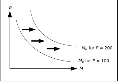
Fig. 13.2: Money market diagram with different prices.
If P increases, the demand for money will increase for all interest rates. This means that the demand curve must be shifted outwards to the right when P increases. Note that with a fixed Y and a fixed money supply, if P increases, R must increase for the money market to remain in equilibrium.
The IS-curve in the AD-AS model
The IS-curve is not affected by P in the AD-AS model
We can define an IS-curve in the AD-AS model in exactly the same way as in the IS-LM model: it will give us all combinations ofR and Y where the goods market is in equilibrium, that is, where aggregate demand is equal to GDP, YD(Y, R) = Y.
Since P does not affect any part of the goods market, P will not affect the IS curve. The IS curve in the AD-AS model is exactly the same as IS-curve in the IS-LM model.
The LM-curve in the AD-AS model
The LM-curve will shift upwards (downward) when P is increases (decreases) in the AD-AS model is moved
The LM-curve in the AD-AS model is slightly more complicated as P will affect the demand for money. In the IS-LM model, the LM-curve is defined as all combination of R and Y where the money market is in equilibrium, that is, where the demand for money is equal to the supply of money, MD(Y, R) = MS.
In the AD-AS model, the LM-curve shows all combinations of R and Y, where the money market is in equilibrium for a given P. For a given P, we can still draw the LM curve in the AD-AS model just as we did in the IS-LM model. For a given P, there are different combinations of R and Y where the money market is in equilibrium. But for another given P,another set of combinations of R and Y will be associated with equilibrium in the money market. This means that the LM-curve will shift when P changes.
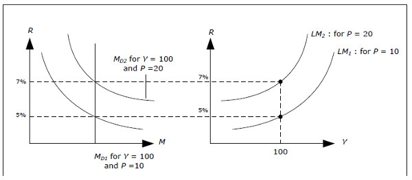
Fig. 13.3: Money market diagram with different prices.
- First consider the top left figure. The demand curve for money, MD1, is drawn for Y = 100 and P = 10. The equilibrium interest rate is R = 5%.
- Y = 100 and R = 5% will provide us with a point on the LM1 curve to the right.
- Now suppose that P increases to 20. We know that the demand for money will increase and the curve will shift to the right (to MD 2).
- We see that R = 5% and Y = 100 is no longer an equilibrium in the money market.
- To the left you see that R = 7% will be an equilibrium when Y = 100 for P = 20.
- R = 7% and Y = 100 must be on a new LM curve (LM2) associated with the higher price P = 20.
There is an LM curve for P = 10 (LM1) and an LM curve for P = 20 (LM2). The important thing to remember is that inthe AD-AS model, there is one LM-curve for each value of P.When P increases, the LM curve will shift to a new curve which will be above the old one. The reason, again, is that R must increase when P increases to keep the money market in equilibrium.
Equilibrium in both the goods and in the money market
If both the goods and the money markets are to be in equilibrium…
…if P increases, Y must fall and R increase ...
…if P decreases, Y must increase and R fall
For a given P , we can use the IS and the LM curves to find the equilibrium values of interest rate and GDP. However, we can also figure out how the equilibrium values of R and Y depend on P.
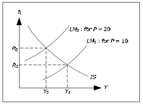
Fig. 13.4: How P affects the equilibrium in the goods and money market.
LM1 is the LM curve when P = 10, while LM2 is the LM curve when P = 20. LM2 is above LM1 as explained in the previous section. IfY1 and R1 are the equilibrium values when P = 10 and Y2 and R2 are the equilibrium value when P = 20, we see that Y2 < Y1 and that R2 > R1.
We may draw the following conclusion. When prices increase, GDP must fall and interest rates must increase if both the goods and the money market is to be in equilibrium. The economic intuition is something like this
- When P increases, the demand for money increases
- When MD increases, the interest rate increases
- When R increases, investments fall
- When I falls, GDP falls
Of less importance is the following point: when GDP falls in step 4, MD will fall slightly – although not as much as it increased in step 1. Therefore, the interest rate will decline somewhat compared to the level in step 2.
More importantly, we no longer have a unique equilibrium from the money market and the goods market. Since there is a unique LM curve for each value of P, there is an equilibrium (in both markets) for each value of P.
The AD curve
The AD curve shows all combinations of P and Y where the goods and the money markets are both in equilibrium. The AD curve slopes downwards.
From the section above, we know that Y must fall if P increases if we want both markets to remain in equilibrium. In this section we derive the exact relationship between Y and P when both markets are in equilibrium.

Fig. 13.5: Derivation of the AD curve.
We can illustrate our derivation using the diagram above.
- First select P1 = 10 and P2 = 20 in the lower diagram.
- Draw the IS curve in the upper diagram and two LM curves – the one corresponding to P = 20 must be above the one for P = 10.
- Identify the resulting GDP in the upper graph for both prices – the highest level of GDP is associated with the lower of the prices.
- Extend these levels of GDP to the lower graph. This will result in two points in the lower graph.
- Keep on doing this with other prices. The resulting downward sloping curve in the lowergraph is called the AD-curve.
Keep in mind that both the goods market and the money market is in equilibrium at all points on the AD curve. Therefore, the AD-curve alone cannot identify to which point the economy will move.
The AD curve is the aggregate demand
The AD curve is the aggregate demand as a function of P when the goods and money market are both in equilibrium
The AD curve shows not only the equilibrium combinations of P and Y – it also shows the aggregated demand as a function of P when both markets are in equilibrium. This follows from the equilibrium condition in the goods market which requires aggregate demand to be equal to GDP. When we change P, the AD curve will tell us the response of Y and therefore also the response of YD. You may therefore use the AD curve to find the aggregate demand for different prices under the condition that both markets are in equilibrium.
Initially, this may seem like a contradiction. In section: Aggregate demand , we claimed that the only endogenous variables that affect aggregate demand where R and Y. Specifically, we stated that P does not affect YD as long as we kept the R and Y fixed.
- If we start in equilibrium and change P but keep R and Y constant, YD will not change but we will not longer be in equilibrium in the money market.
- If we require both markets to be in equilibrium, R and Y must change when P changes.
- Specifically, R must fall and Y must increase when P decreases if both markets are to be in equilibrium.
- Since YD depends positively on Y and negatively on R, YD will then increase.
- Thus, YD increases when P falls when both markets remain in equilibrium and there is no contradiction.
Aggregate supply
In order to determine all the variables in the AD-AS model, we need one more equilibrium condition so that we can identify a unique point on the AD curve as the unique equilibrium. This condition will come from the production side and the labor market.
The Labor Market
In the AD-AS model, the economy will always be on the response curve – the thick line in the chart below.
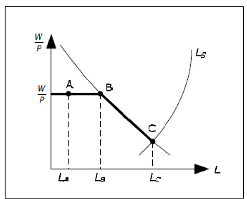
Fig. 13.6: The labor in the AD-AS model.
The response curve has a horizontal part and a downward sloping part. In the IS-LM model, we had only the horizontal since real wages where constant. We could not move beyond LB.
We can explain the response curve by examining the economy moving from point A to point C.
- First, the economy is at point A, with prices P, wages W, real wages W/P and amount of labor LA. The profit-maximizing quantity of labor is LB but firms do not choose this quantity due to lack of demand.
- If aggregate demand increases, L may increase without P being affected, up to L = LB. To the left of point B, the IS-LM model is fully sufficient and the AD-AS model is redundant.
- When L = LB, L cannot increase without real wages falling. In the AD-AS model, real wages are reduced by an increase in P (with W constant) and we begin to move down the demand curve for labor.
- Between the points B and C, L will increase when P increases.
- However, we cannot increase L above LC. When we are at point C, not even a price increase will help. Real wages are no so low that the labor supply sets the limit - there are no more people that want to work for these low real wages.
Let us summarize:
- As long as L is smaller than LB, L may change with no change in prices. In this range, there is no relation between P and L.
- When L is between LB and LC, then L increases with P.
- L can never be greater than the LC.
The chart below shows the relationship between L and P
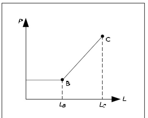
Fig. 13.7: The relationship between L and P.
Aggregate supply and the AS curve
The AS curve is the aggregate supply as a function of P. It is horizontal when the supply is low and upward sloping when the supply is high.
From the relationship between L and P we can derive the relationship between YS and P as YS is determined by L by the production function (the higher L, the higher the the ).
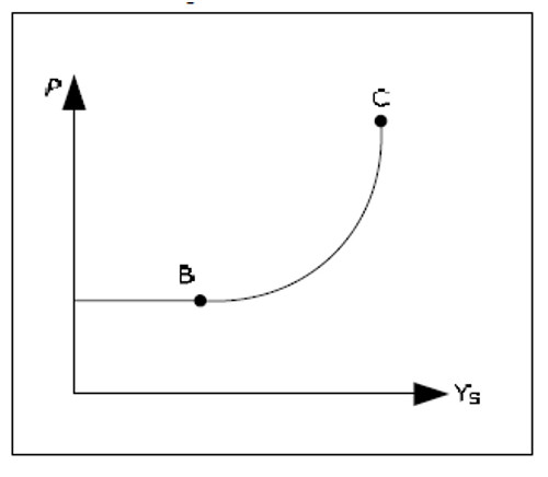
Fig. 13.8: The relationship between YS and P.
Between points A and B prices are constant and firms produce an amount exactly equal to the aggregate demand. Here, the reversed Say's Law and the IS-LM model apply. In this interval, the ASAD model is redundant. Between points B and C we have a positive relation between P and YS.
Neither the reversed Say's Law nor the IS-LM model apply. It is, however, unreasonable to believe that there would be a "sharp edge" in the relationship between L and P and between YS and P in the real economy. The schedules are drawn this way to simplify the explanation. A more reasonable assumption would be that the relationships are smooth curves.
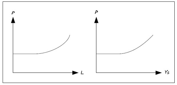
Fig. 13.9: More realistic relationships between L and P and between YS and P.
Determination of all the endogenous variables in the AD-AS model
Determination of P and Y
Prices and GDP are in equilibrium when aggregate supply is equal to the aggregate demand in the AD-AS model
We know that for all points on the AD curve, both the goods and money market are in equilibrium. We also know that firms will always produce an amount consistent with the AS-curve.
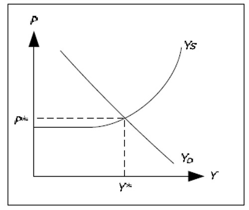
Fig. 13.10: Determination of P and Yin the AD-AS model.
There is only one level for P and for Y which is consistent with equilibrium in both markets and which is consistent with firm behavior. The price level at this point is the equilibrium price level and the GDP level at this point is the equilibrium quantity of GDP. We denote these levels by P* and Y*.
The AD-AS model , P will always move towards P* and Y will always move towards Y*. To justify this behavior of the economy, let us consider what will happen if P < P*.
- From the graph, we see that in this case YS < YD.
- Since we are on the upward sloping part of the AS-curve, aggregate supply will notautomatically increase. But since firms can sell everything they produce and since stocks are diminishing, they will raise prices.
- When P increases, real wages W/P falls and L increases. With more labor, firms can increase production.
- When P increases, the demand for money will increase. Interest rates will then increase and YD will fall (the LM-curve shifts upwards).
- Overall, YS increases and YD falls when P increases. As long YS < YD, firms will continue to raise prices. Thus, prices will continue to increase until YS = YD and the economy is in equilibrium.
Determination of other variables
Once P and Y are determined, all other endogenous variables will be determined as well. The interest rate is determined by money market diagram and the components of GDP are either exogenous or they depend on R or Y. W is constant and since P is determined, so is the real wage. Then L and the unemployment rate is determined as well.
Note that although this diagram is looks exactly like the "standard supply and demand curves” for a single good from microeconomics, the derivation and interpretation is very different.
The equations of the AD-AS model
To summarize the AD-AS model, we can look at its equations. The IS-LM model was "solved" by simultaneously solving the equations
YD(Y, R) = Y
MD(Y, R) = MS
for Y and R. Since MS was exogenous, we had two equations and two unknown and the system of equation could be solved. The solution was illustrated by the IS-LM diagram.
In the AD-AS model, the situation is slightly more complicated because MD now depends on three variables: Y, R and P. We can no longer solve
YD(Y, R) = Y
MD(Y, R, P) = MS
for Y, R and P as we have three unknowns and only two equations. We need an additional equation in the AD-AS model. The third equation in the AD-AS model comes from the production function and the labor market. We showed that L depends on P and since YS depends on L, YS will depend on P. Equilibrium requires that their supply equals actual production, i.e., YS(P) = Y. The three equations of the AD-AS model are therefore
YD(Y, R) = Y
MD(Y, R, P) = MS
YS(P) = Y
These are to be solved for Y, R and P. The solution is illustrated in the AD-AS diagram, where the first two equations are summarized in the AD curve YD(P) = Y.
Note how the three different versions of the Keynesian model we have studied so far are related to the number of variables / equations.
- In the Keynesian cross model, we have only one variable (Y) and an equation: YD(Y) = Y.
- In the IS-LM model, we have two variables (Y and R) and two equations: YD(Y, R) = Y and MD(Y, R, P) = MS.
- In the AD-AS model, we have three variables (Y, R, P) and three equations: YD(Y, R) = Y,
- M (Y, R, P) = MS och YS(P) = Y.