A First Look at Investments
- Details
- Category: Finance
- Hits: 6,810
Historical Rates of Return Background and Market Institutions
The subject of investments is so interesting that I first want to give you a quick tour, instead of laying all the foundations first and showing you the evidence later. I will give you a glimpse of the world of historical returns on the three main asset classes of stocks, bonds, and 'cash," so that you can visualize the main patterns that matter—patterns of risk, reward, and co variation.
This chapter also describes a number of important institutions that allow investors to trade equities.
Stocks, Bonds, and Cash, 1970-2010
Financial investments are often classified into just a few broad asset classes. The three most prominent such classes are cash, bonds, and stocks.
Cash : The name cash here is actually a misnomer because it does not designate physical dollar bills under your mattress. Instead, it means debt securities that are very liquid, very low-risk, and very short-term. Other investments that are part of this generic asset class may be certificateof deposits (CDs), savings deposits, or commercial paper. (These are briefly explained in Book Appendix A.) Another common designation for cash is money market. To make our life easy, we will just join the club and also use the term "cash."
Bonds : These are debt instruments that have longer maturity than cash. You already know much about bonds and their many different varieties. I find it easiest to think of this class as representing primarily long-term Treasury bonds. You could also broaden this class to include bonds of other varieties, such as corporate bonds, municipal bonds, foreign bonds, or even more exotic debt instruments.
Stocks : Stocks are sometimes all lumped together, and sometimes further categorized into different kinds of stocks. The most common such sub classification for U.S. domestic stocks is as follows:
The asset class containing a few hundred stocks of the largest firms that trade very frequently is often called large-cap stocks. (Cap is a common abbreviation for capitalization.) Although not exactly true, you can think of the largest 500 firms as roughly the constituents of the popular S&P 500 stock market index, (S&P is Standard and Poor's, the company which invented this index in 1923 and continues to maintain it, Stocks continuously change in value, disappear, etc-) Our chapter focuses mostly on these large cap S&P 500 stocks and often just calls them "stacks."
There are a few thousand other stocks. They are also sometimes put into multiple categories, such as "mid-cap" or "small-cap." Inevitably, these stocks tend to trade less often, and some seem outright neglected. Small caps can be really small. They may have only $10 million in market cap, and not a single share may be traded for days at a time, In any case, it is so expensive to trade most small-cap stocks that large investors do not bother with them.
There are also other stock-related subclasses, such as industry stock portfolios, or a classification of stocks into -value firms" and "growth firms," and so on. We shall ignore everything except the large-cap stock portfolio.
Do not take these categories too literally. They may not be representative of all assets that would seem to lit the designation. For example, most long-term bonds in the economy behave like our bond asset class, but some long-terra corporate bonds behave more like stocks, Analogously, a particular firm may own a lot of bonds, and its rates of return would look like those on bonds and not like those on stocks.
It would also be perfectly reasonable to include more or fewer investments in these three asset classes. (We would hope that such modifications would alter our insights only a little bit.) More importantly; there are also many other important asset classes that we do not even have time to consider, such as real estate, hedge funds, financial derivatives, foreign investments, or art. Nevertheless, cash, bonds, and stocks (or subclasses thereof) are the three most studied financial asset classes, so we will begin our examination of investments by looking at their historical performances.
Graphical Representations of Historical Returns for the S&P 500 Sian with Exhibit 7.1. It shows the year-by-year rates of return (with dividends) of the S&P 500. Actually, because of how different sources treat dividends (reinvest or not?), the numbers are never exact. Some sources even omit dividends, which is definitely wrong.
The series we are using take dividends into account. (All the numbers we are using are posted on the book's website. Obviously, do not want to write this textbook with 8 decimal points of precision, so please be aware of and do not worry about rounding errors in any of the calculations that follow.) The table and the plot illustrate the same data:
You would have earned 3.5% in 1970, 14.1% in 1971, 18.7% in 1972, -14.5% in 1973, and so on. The average rate of return over all 41 years was 11A% per annum—which I marked with a blue triangle on the left side and the dot-dashed line.
Exhibits 7.2 and 7.3 take the same data as Exhibit 7.1 but present it differently. Exhibit 7.2 shows a histogram that is based on the number of returns that fall within a range. This makes it easier to see how spread out returns were—how common it was for the S&P 500 to perform really badly, perform just about okay, or perform really well.
For example, the table in Exhibit 7.1 shows that 8 years (1971, 1972, 1979, 1982, 1986, 1988, 2004, and 2006) had rates of return between 10% and 20%. In our 41 years, the most frequent return range was between 0% and 10%. Yet there were also many years that had rates of return below 1091—and even three years in which you would have lost more than 20% of your money (1974, 2002, and 2008). Again, the blue triangle indicates that the average rate of return was 11.4%.
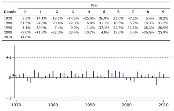
Exhibit 7.1: The Time Series of Rates of Return on the S&P 500, 1970-2010.
The time-series graph is a representation of the rates of return of the S&P 500 index (including dividends), as shown in the table above.
The average rate of return was 11.4% (indicated by the blue triangle and the dot-dashed line); the standard deviation was 17.7%. Original source of data for all applicable figures in this chapter: Ibbotson Stocks, ponds, Bills and inflation, SBBI Valuation Yearbook, Morningstar 2011.
Most investors are not interested in statistics as much as they are interested in how much money they would have ended up with. Can you take $1 and the 11.4% average return, and use the compounding formula? Well, this would indicate a payoff of $1 - 1.11441 -1 P:v $82.62 in 2010. Unfortunately, you would have been far off the mark.
Instead, you need a graph of the compound rate of return, which is in Exhibit 7,3. It plots the compounded annual returns (on a logarithmic scale). For example, by the end of 1973, the compound return of $1 invested in 1970 would have been
$1 • (1 + 3,5%) • (1 + 14,1%) • (1 + 18.7%) • (1 - 14,5%) as $1,20 P111#9 (1 + rpm) • (1 + rj971) • (1 + r1973) • (1 -I- 1-1973) P12/31/73
If you do this for all 41 years, you end up with $46.80, much less than the naive $82,62.
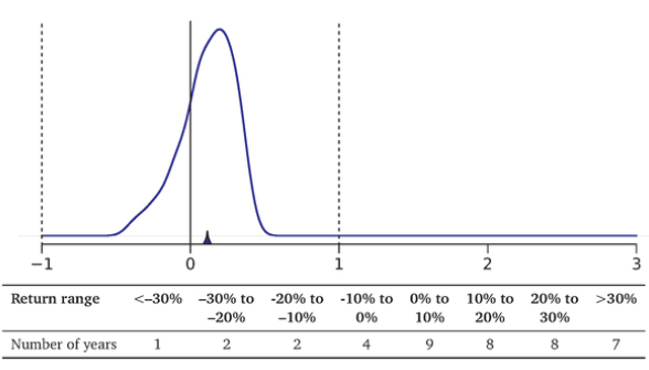
Exhibit 7.2: The Srarisricai Distribution Function of S&P 500 Rates of Return, 1970-2010.
The graph and table are just different representations of the data in Exhibit 7.1. Formally, this type of graph is called a density function. It is really just a smoothed histogram.
Thus, many long-term investors are misled by the more common arithmetic average rate of return—commonly just called the mean or average. What is the intuition? For example, think of a rate of return of -50% (you lose half) followed by +100% (you double), It has the intuitively correct geometric net return of zero. However, the average rate of these two returns is a positive (-50%+10.0%)/2 +25%, dikes. Unfortunately, there is no simple way to convert an arithmetic rate of return into a geometric rate of return (or an annualized rate of return). You will later even see a real-world example in which the geometric rate of return was -100% and the average rate of return was positive.
The annualized compound rare of return is sometimes called a geometric average. To compute the geometric average, you un compound. The annualized rate of return from 1970-2010 (41 years) was

The arithmetic rate of return of 11.4% was 1.6% higher. This is the rate of return that is relevant for a (long-term) buy-and-hold investor. There is one novel aspect to this graph, which is the gray shaded area, It marks the cumulative CPI inflation.
The purchasing power of $1 in 1970 was about the same as $5.79 in 2010. Thus, the
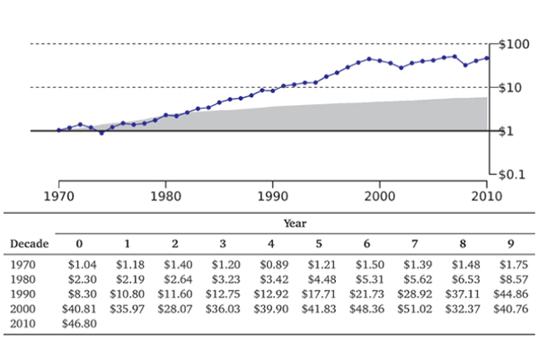
Exhibit 7.3: Compound Rates of Return for the S&P 500, 7970-2010 ,
This graph and table are again just different representations of the same data in Exhibit 7.1. The gray area underneath the figure is the cumulative inflation-caused loss of purchasing power.
$46.80 nominal value at the end of 2010 was really only worth $46.80/$5.79 ft $3.08 in 1970 inflation-adjusted dollars, (And, of course, none of these figures take taxes into account.)
The annualized holding rate of return cannot be inferred from the average annual rate of return, and vice versa. The two are identical only if all rates of return are the same (i.e., when there is no risk). Otherwise, the geometric rate of return is always less than the arithmetic rare of return. (And the more risk, the bigger the difference.)
Historical Performance for a Number of Investments Stocks, Bonds, and Cash
What does history tell you about rare of return patterns on the three major investment categories—stocks, bonds, and cash? You can find out by plotting exactly the same graphs as those in Exhibits 7.1, 7.2, and 7.3. Exhibit 7.4 repeats them for cash, bonds, and stocks all cm the same scale, You have already seen the third row, but I have changed the scale to make it easier to make direct comparisons to the other two asset classes, These mini-graphs display a lot of information about the performance of these investments,
So let's compare the first three rows:
Cash in the first row is the overnight Federal Funds interest rate. Note how tight the distribution of cash returns was around its 5.7% mean. You would never have lost money nominal terms), but you would rarely have earned much more than its mean.
The value of your total investment portfolio would have steadily marched upward—although pretty slowly. Each dollar invested in January 1970 would have become $9.59 at the end of 2010. Of course, inflation would have eroded the value of each dollar. In purchasing power, your $1 in 1970 was equivalent to $5.79 in 2010. Therefore, the $9.59 investment result in cash would have only been worth about $9.59/$5.79 $1.66 in 1970 inflation-adjusted dollars. Over 41 years, you would not even have doubled your real purchasing power.
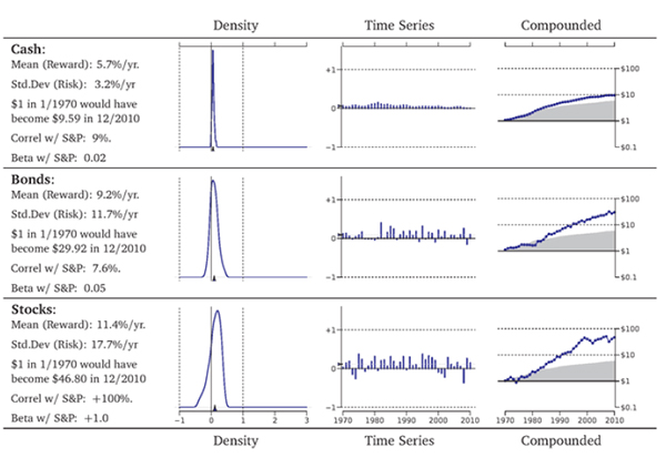
Exhibit 7.4: Comparative Investment Performance, 1970-2010.
Bonds in the second row are long-term Treasury bonds. The middle graph shows that the bars are now sometimes slightly negative (years in which you would have earned a negative rate of return)—but there are now also years in which you
would have done mud' better than cash. This is why the histogram is much wider for bonds than it is for cash: Bonds were riskier than cash. The standard deviation tells you that bond risk was 11.7% per year, much higher than the 3.2% cash risk.
Fortunately, in exchange for carrying more risk, you would have also enjoyed an average rate of return of 9,2% per yea; which is a lot more than the 5,7% of cash. And $1 invested in 1970 would have become not just the $9.59 in 2010 (cash), but $29.92 ($5.17 in real terms).
Stock Market in the third row is a portfolio of the S&P 500 firms. (Returns are calculated with dividends.) The left graph shows that large stocks would have been even riskier than bonds. The stock histogram is more 'spread out' than the bond histogram_ The middle graph shows that there were years in which the negatives of stocks could be quite a bit worse than those for bonds, but that there were also many years that were outright terrific. And again, the higher risk of
stocks also came with more reward. The S&P 500's risk of 17.7% per year was compensated with a mean rate of return of 11.4% per year. Your $1 invested in 1970 would have ended tip being worth $46.80 in 2010 ($8.08 in real terms).
The difference between $46.80 in stocks and $9.59 in cash or $29.92 in bonds is an understatement if you are a common taxable retail investor in a high tax bracket.
Nominal interest payments would have been taxed each year at your full income tax rate, between 30% and 50% per year, In contrast, the capital gains on stocks would have been taxed only at the end and at the much lower capital gains tax rate, between 15% and 30%. Roughly speaking, taking taxes into account, if you had invested in cash, you would not have ended up with more real purchasing power than you started with, You would have gained a little bit of real purchasing power in bonds (maybe $1.50-$2.00).
And you would have roughly quadrupled your purchasing power in stocks. This was a great-and perhaps even unusually great-41 years for stocks? Not every historical 41-year period would have shown as large a difference between cash, bonds, and stocks.
Other Asset Classes
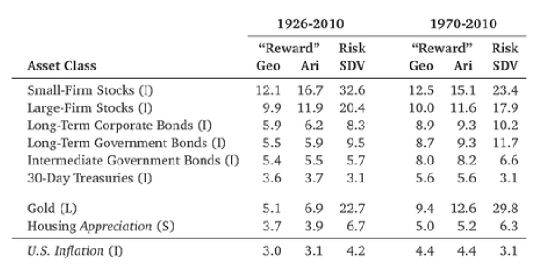
Exhibit 7.5: Comparative investment F'erforinance, 2970-2010,
Original data sources: See leftmost column: L= London Gold Exchange, 1=Ibbotson Stocks, Bonds, Bills and Inflation, SBBI Valuation Yearbook, /viorningstar 2011. 5=- Robert Shiller, Irrational Exuberance, 2nd Ed, Note that housing appreciation ignores the useful housing rental yield, and thus understates the rate of return.
Exhibit 7.5 shows the performance of a few other large asset classes and over a longer time period, too. Small-firm stocks were riskier (and more difficult to trade), but their average rate of return was higher Corporate bonds sit between government bonds and stocks in terms of reward, although their risk was comparable to the former.
Intermediate government bonds (i.e„ with about 5-year maturity) were somewhere between cash and long-term bonds. Gold was anextremely risky investment by itself, but it also did well over the sample. (Not shown in this table, it did well in years when stocks did poorly.) Moreover, unlike bonds, gold's gains were taxed at the lower capital-gains rate. Housing is the average price appreciation of residential houses. It probably understates the rate of return by about 3-6% per year, because it omits the value and other costs of living in a house.
Owning a house from 1970 to 2010 was a good investment, especially if you take into account that tax rules now shelter most gains from any taxes, However, the 6-7% risk may be a bit misleading. Many economists believe that there was a housing bubble in the 2000's, which explains both the fantastic appreciation and the subsequent crash. From 1992 to 2006, there was not a single year in which prices declined. But from 2007 to 2009, residential houses lost about 30% of their values.
Individual Stocks
Instead of holding entire asset classes, you could also have purchased just an individual stock. How would such holdings have differed from an investment in the broader asset class "stocks"? Exhibit 7.6 keeps the same scale but now shows the rates of return of a few sample stalwart Finns: Coca-Cola [MI PepsiCo [PEP], Sony [SINE], and United Airlines [UAL]. For comparison, the bottom is again the S&P 500. You can see that individual stocks' histograms are really wide.
Investing in a single stock would have been a rather risky venture, even for these four household names. Indeed, it is not even possible to plot the final year for UAL in the rightmost compound return graph, because UAL stock investors lost all invested money in the 2003 bankruptcy, which
on the logarithmic scale would have been minus infinity, And UAL illustrates another important issue: Despite losing all the money, it still had a positive average rate of return.
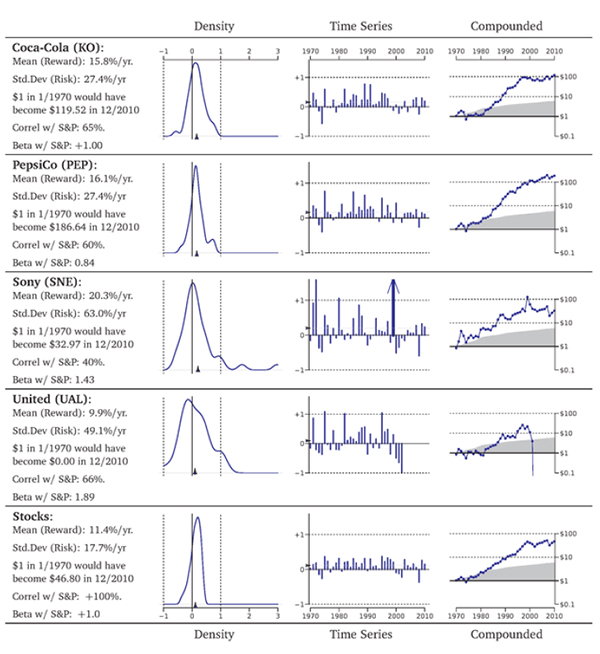
exhibit 7.6: Comparative Investment Performance,
7970.2010. The arrow for Sony indicates a return of 300% in 1999. The original data source for individual stock returns was CRSP
Comovement, Market Beta, and Correlation
Exhibit 7.7 highlights the rates of return on the S&P SOO and one specific stock, PepsiCo (PEP). The bottom row redraws the time-series graphs for these two investments (history in the top row). Do you notice a correlation between these two series of rates of return?
Are the years in which one is positive (or above its mean) more likely also to see the other be positive (or above its mean), and vice versa? It does seem that way. For example, the worst rates of return for both are 1974. Similarly, 1973 and 2002 were
bad years for investors in either the S&P 500 or PepsiCo, In contrast, 1975, 1985. 1989. and 1995 were good years for both. The correlation is not perfect: In 1999, the S&P SOO had a good year, but PepsiCo had a bad one; and in 2000, the market had a bad
year, but PepsiCo had a good one. It is very common for all sons of investments in the economy to move together with the stock market: In years of malaise, almost everything tends to be in malaise, In years of exuberance, almost everything tends to be exuberant.
This tendency is called comovement. The comovement of investments is very important if you do not like risk. An investment that increases in value whenever the rest of your portfolio decreases in value is practically like "insurance" that pays off when you need it most You might buy into such an investment even if it offers only a very low expected rate of return.
In contrast, you might not like an investment that does very badly whenever the rest of your portfolio also does badly. To be included in your portfolio, such an investment would have to offer a very high expected rate of return.
How can you measure the extent to which securities covary with others? For example, how does PepsiCo covary with the S&P 500 (our stand-in for the market portfolio)? Did PepsiCo also go down when the market did (making a bad situation worse), or did it go up (thereby serving as useful insurance)? How can you quantify such comovement?
You can answer this graphically. Plot the two return series against one another, as is done in the bottom plot in Exhibit 7,7, Then find the line that best fits between the rihra. series. (You will learn later how to compute it.) The slope of this line is called the market beta of a stock, and it is a measure of comovement between the rate of return on the stock with the rate of return on the market. It tells an investor whether this stock moved with or against the market. It carries great importance in financial economics.
- If the best-fitting line has a slope that is steeper than the 45° diagonal (well, if the x- and y-axes are drawn with the same scale), then the market beta is greater than Such a line would imply that when the stock marker did better (the x-axis), on average your stock did a tat better' (the y-axis), For example, if a stock has a very steep positive slope—say, +3—then (assuming you hold the market portfolio) if the market dropped by an additional 10%, this stock would have been expected to drop by an additional 30%. If you primarily held the market portfolio, this new stock would have made your bad situation worse.
- If the slope is less than 1 (or even 0, a plain horizontal line), it means that, on average, your stock did not move as much (or not at all) with the stock market.
- If a stock has a very negative slope such as –2, this investment would likely have "rescued" you when the market dropped by 10%. On average, it would have earned a positive 20% rate of return, Adding such a stock to your market portfolio would be like buying insurance.
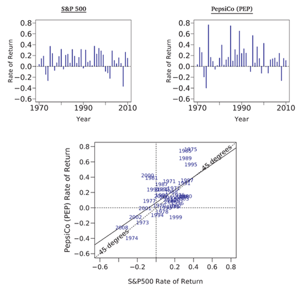
Exhibit 7.7: Rates of Return on the S&P 500 and PepsiCo. (PEP), 1970-2010.
The top left graph plots the annual rate of return on the S&P 500; the top right graph plots the annual rate of return on PepsiCo. The bottom graph combines the information. The stock market rate of return is on the x-axis, the PepsiCo rate of return is on the y-axis.
The figure shows that in years when the stock market did well, PepsiCo tended to do well, too, and vice versa. This can be seen in the slope of the best-fitting line, which is called the market beta of PepsiCo. The market beta will play an important role in investments. Real-world Advice: In practice, it is better to compute a market beta from the most recent 3 years of daily stock return data, and not from 41 years of animal stock return data, as I have done in this figure.
PepsiCo's particular line had a slope of 0_84_ That is, it was a little less steep than the diagonal line. In effect, this means that if you had held the stack market, PepsiCo would have been neither great insurance nor a great additional hazard for you. A 1% performance above (below) normal for the S&P would have meant you would have expected to earn 0,84% above (below) normal in your PepsiCo holdings.
Instead of beta, you could measure comovement with another statistic that you may already have come across: the so-called correlation. Correlation and beta are related.
The correlation has a feature that beta does not. A correlation of +100% indicates that two variables always perfectly move together; a correlation of 0% indicates that two variables move about independently; and a correlation of –100% indicates that two variables always perfectly move in opposite directions, (A correlation can never exceed +100% or –100%.) In PepsiCo's case, one can work out that the correlation is +60%.
The correlation's limited range from –1 to +1 is both an advantage and a disadvantage. On the positive side, the correlation is a number that is often easier to judge than beta. On the negative side, the correlation has no concept of scale. It can be 100% even if the y variable moves only very, very mildly with x (e.g,, if every y = 0_0001 x, the correlation is still a positive 100%)- In contrast, beta can be anything from minus infinity to plus infinity
A positive correlation always implies a positive beta, and vices versa, Of course, beta and correlation are only measures of average comovement: Even for investments with positive betas, there are individual years in which the investment and stock market do not move together (look back at 1999 and 2000 for PepsiCo and the S&P 500). Stocks with negative betas, for which a negative market rate of return an average associates with a positive stock return (and vice versa), are rare. There are only a very few investment categories that are generally thought to be negatively correlated with the market—principally gold and other precious metals.
The Big Picture Take-Aways
What can you learn from these graphs? Actually, almost everything there is to learn about investments! I will explain these facts in much more detail soon. In the meantime, here are the most important points that the graphs show:
- History tells us that stocks offered higher average rates of return than bonds, which in turn offered higher average rates of return than cash, However, keep in mind that this was only on average. In any given year, the relationship might have been reversed_ For example, stock investors lost 22% of their wealth in 2002, while cash investors gained about 1.7%.
- Although stocks did well (on average), you could have lost your shirt investing in them, especially if you had bet on just one individual stock. For example, if you had invested in United Airlines in 1970, you would have lost all your money
- Cash was the safest investment—its distribution is tightly centered around its mean, so there were no years with negative returns. Bonds were riskier. And stocks were even riskier (Sometimes, stocks are said to be "noisy," because it is really difficult to predict how they will perform.)
- There seems to be a relationship between risk and reward: Riskier investments tended to have higher average rates of return. (However; you will learn soon that risk has to be looked at in context, Thus, please do not overread the simple relationship between the mean and the standard deviation here,)
- Large portfolios consisting of many stocks tended to have less risk than individual stocks. The S&P 500 stocks had a risk of around 15-20% per year, which was less than the risk of most individual stocks (e.g., PepsiCo had a risk of about 27%). This is due to the phenomenon of diversification.
- The average rate of return is always larger than the geometric (compound) rate of return. A positive average rate of return usually, but not always, translates into a positive compound holding rate of return. For example, United Airlines had a positive average rate of return, despite having lost all its investors' money.
- Stocks tend to move together. For example, if you look at 2001 and 2002, not only did the S&P 500 go down, but all the individual stocks tended to go down, too. In 1998, on the other hand, most stocks tended to go up (or at least not down much). The mid-1990s were good to all stocks. In contrast, money market returns had little to do with the stock market. Long-term bonds were in between.
- On an annual frequency, the correlation between the stock market and either cash or long-teen bands (the S&P 500) was about 10%. The correlation between individual stocks and the stock market was around 50% to 70'i1 The fact that investment rates of return tend to move together is important. It is the foundation for the market beta, a measure of risk that we have touched on and that will be explained in detail in Chapter 8.
Will History Repeat Itself?
As a financier, you are not interested in history for its own sake. instead, you really want to know more about the future. History is useful only because it is your best available indicator of the future. But which history? One year? Thirty years? One hundred years? I can tell you that if you had drawn the graphs beginning in 1926 instead of 1970, the big conclusions would have remained the same. However, if you had started in 2001, things would have been different.
What would you have seen? Four awful years for stock investors. You should know intuitively that this would not have been a representative sample period. To make any sensible inferences about what is going on in the financial markers, you need many years of history, not just one, two, or three—and certainly not the 6-week investment performance touted by some funds or friends (who
also often display remarkable selective memory!). The flip side of this argument is that you cannot reliably say what the rate of return will be over your next year. It is easier to forecast the overage annual rate of return over five to ten years than over one year.
Your investment outcome over any single year will be very noisy Instead of relying on just one year, relying on statistics computed over many years is much better. However, although twenty to thirty years of performance is the minimum number necessary to learn something about return patterns, this is still not sufficient for you to be very confident. Again, you are really interested in what will happen in the next five to ten years, not what happened in the last five to ten years. Yes, the historical
performance can help you judge, but you should not trust it blindly. For example, an investor in UAL in 2000 might have guessed that the average rate of return for UAL would have been positive—and would have been sorely disappointed. Investors in the Japanese stock market in 1986 saw the Nikkei-225 stock market index rise from 10,000 to 40,000 by 1990—a 40% rate of return per year. If they had believed that history was
a good guide, they would have expected 40,000 , 1,4013 sus 3,2million by the end of 2002. Instead, the Nikkei had fallen below 8,000 in April 2003 and has only recently recovered to 15,307 by December 2010, History would have been a terrible guide.
Nevertheless, despite the intrinsic hazards in using historical information to forecast future returns, having historical data is a great advantage. It is a rich source of forecasting power, so like everyone else, you will have to use historical statistics. But please be careful not to rely too much on them_ For example, if you look at an investment that had extremely high or low past historical rates of return, you may not want to believe that this is likely to continue.
In relative terms, what historical information can you trust more and what historical information should you trust less?
Historical risk : Standard deviations and correlations (how stock movements tend to be related or unrelated) tend to be fairly stable, especially for large asset classes and diversified portfolios. That is, for 2010 to 2020, you can reasonably expect PepsiCo to have a risk of about 25-30% per year, a correlation of about 50-70% with the market, and a market beta of about 0.7 to 1,1.
Historical mean reward : Historical average rates of return are not very reliable predictors of future expected rates of return. That is, you should not necessarily believe that PepsiCo will continue to earn an expected rate of return of 16% per year.
Realizations : You should definitely not believe that past realizations are good predictors of future realizations. Just because PepsiCo had a rate of return of 10% in 2010 does not make it likely that it will have a rate of return of 10% in 2011.
A lottery analogy may help you understand the last two points better. If you have played the lottery many times, your historical average rate of return is unlikely to be predictive of your future expected rate of return—especially if you have won it big at least once.
Yes, you could trust it if you had millions of historical realizations, but you inevitably do not have so many Consequently, your average historical payoff is only a mediocre predictor of your next week's payoff. And you should definitely not trust your most recent realization to be indicative of the future. Just because "5, 10, 12, 33, 34, 38" won last week does not mean that it will likely win again.
Henceforth, like almost all of finance, we will just assume that we know the statistical distributions from which future investment returns will be drawn. For exposition, this makes our task a lot easier.
When you want to use our techniques in the real world, you will usually collect historical data and pretend that the future distribution is the same as the historical distribution. (Some investors in the real world use some more sophisticated techniques, but ultimately these techniques arc also just variations on this theme.) However, always remember: historical data is an imperfect guide to the future.