General Equilibrium
- Details
- Category: Microeconomics
- Hits: 8,118
When we have studied equilibria so far, it has always been so-called partial equilibria. (A partial equilibrium is one where we assume that “everything else is unchanged.”) However, we have also seen that a change in one variable can lead to changes in many other variables, so the restriction that everything else is unchanged may not be very realistic.
For example, a price change can affect the price of close substitutes and complementary goods. We will now study how interactions between two individuals in a very simple economy lead to general equilibrium, i.e. a simultaneous equilibrium in all markets.
A "Robinson Crusoe" Economy
Consider an economy with only two agents on a desert island: Robinson and Friday. Those two are then the only consumers and the only producers. Let us assume that they also produce only two goods: Coconuts and fish. The question is then how much coconuts and fish to produce, and how to allocate them among themselves.
Efficiency
We have already mentioned efficiency several times in this posts (for instance in The Deadweight Loss of a Monopoly). Efficiency is about how much waste there is in an economy; less waste means more efficient. There are several related ways to define efficiency. An often-used measure of efficiency regarding allocations is Pareto efficiency. The definition of Pareto efficiency is:
Pareto improvement. A change in allocation such that
- No one is worse off; and
- At least one, possibly several, is better off.
Pareto efficient or Pareto optimal. An allocation such that
- No Pareto improvements are possible.
The Edgeworth Box
In Chapter 3, we discussed the basics of consumer theory. We described, for instance, indifference curves and the budget line. If we consider an exchange economy in which the quantities of the goods are fixed, we have a zero-sum game. This means that one individual can only get quantities that the other ones do not get; there is, for instance, no growth in the economy. The name “zero-sum game” comes from the fact that, the sum of what some people gain and what others lose is always zero.
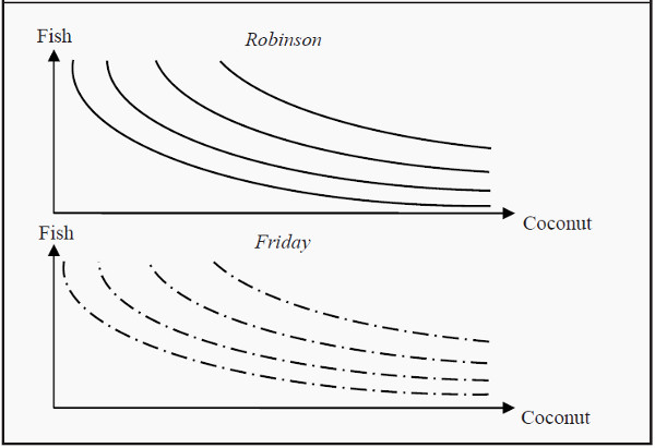
Figure 18.1: Two Indifference Maps
Suppose that Robinson and Friday have different preferences over coconuts and fish, and that these look like in Figure 18.1. Since the quantities of the two goods are fixed, we can combine these two indifference maps into one by taking one of them, for instance Fridays, turning it upside-down and putting it over Robinson’s. We then get a picture such as the one in Figure 18.2. (The additional information in the figure will be explained below.) Such a diagram is called an Edgeworth-box .
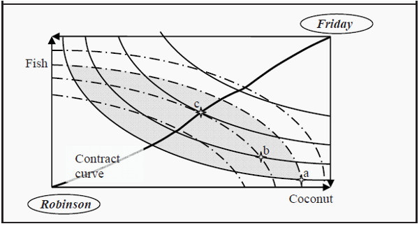
Figure 18.2: An Edgeworth Box for Consumption
Note that the scales in the Edgeworth box are in opposite direction for the two agents. Upwards along the Y-axis, Robinson gets more fish while Friday gets less. To the right along the X-axis, Robinson gets more coconuts and Friday gets less. Also, be aware of which preference curves belong to which individual:
The full lines belong to Robinson while the broken lines belong to Friday.
Efficient Consumption in an Exchange Economy
The clever thing with the construction in Figure 18.2 is that we can see directly which allocations of goods that are Pareto efficient.
- Consider, for instance, point a. Can it correspond to an efficient allocation? Compare it to point b. In b, both Robinson and Friday are better off (as both are on a higher indifference curve). Consequently, b is a Pareto improvement as compared to a, and then a cannot be an efficient allocation. Note that all points within the grey area are Pareto improvements as compared to a.
- Is then point b efficient? Compare b to c. In c, Robinson is better off while Friday is indifferent between b and c. Consequently, c is a Pareto improvement as compared to b, and then b cannot be efficient either.
- In point c, One of Robinson’s indifference curves just barely touches one of Friday’s indifference curves. That is the criterion for a Pareto efficient allocation of goods. Compared to c, every other allocation makes either Robinson or Friday (or both) worse off. c is consequently a Pareto efficient allocation.
Remember that the slope of an indifference curve is the same thing as the marginal rate of substitution; MRS. The criterion for an efficient allocation of goods can then be written
MRS r = MRS f
where the subscripts refer to Robinson and Friday, respectively. In other words, for the allocation to be efficient, both agents are required to have the same marginal valuation of the goods.
Point c is, however, not the only Pareto efficient allocation in the diagram. We could repeat the procedure above for every possible indifference curve, and find all points of tangency. If we would do that, and then connect all points to a curve, we would get the so-called contract curve.
If we assume that the initial allocation of coconuts and fish is as in point a and that we have free trade, then we would expect Robinson and Friday to start trading until they end up somewhere on the contract curve. Moreover, since only points in the grey area are Pareto improvements compared to a, we would expect them to end up on the part of the contract curve that lies within that area. Exactly where we they end up is, however, a question about negotiations between Robinson and Friday.
The Two Theorems of Welfare Economics
There are two important theorems regarding efficiency and competitive markets: the two welfare theorems:
- 1st theorem of welfare economics: If all trade occurs in perfectly competitive markets, the allocation that arises in equilibrium is efficient.
- 2nd theorem of welfare economics: Each point along the contract curve is a competitive equilibrium for some initial allocation of goods.
The first theorem is a variation of “the invisible hand” (see: Properties of the Equilibrium of a Perfectly Competitive Market ). It is enough to have a perfect competition to get an efficient allocation. The second theorem states that there is no loss to efficiency from a reallocation. A competitive market will always find an efficient allocation.
Efficient Production
Regarding production, we can perform an analysis that is very similar to the one we did for consumption. Instead of two indifference maps, we put two isoquant maps (see Production in the Long Run ) together. We imagine that Robinson and Friday have two firms, one that produces coconuts and one that produces fish. In the production, they use labor and capital, and their access to these input factors is fixed.
They have a certain number of fishing tools, tools to pick coconuts with, and a maximum number of working hours. This allows us to construct an Edgeworth box for production (see Figure 18.3).
Let us start by assuming that Robinson and Friday have chosen point a. They consequently invest quite a large number of working hours, but not so much capital, on fishing and, vice versa, a small number of working hours but quite much capital on picking coconuts.
Point a is not efficient. If they instead choose point b, they get, employing the same total number of working hours and the same total amount of capital, more coconuts and just as much fish as they did in a. If they would choose point c instead of a, they get more fish and just as many coconuts as they did before. Consequently, both point b and c constitute efficiency gains compared to point a.
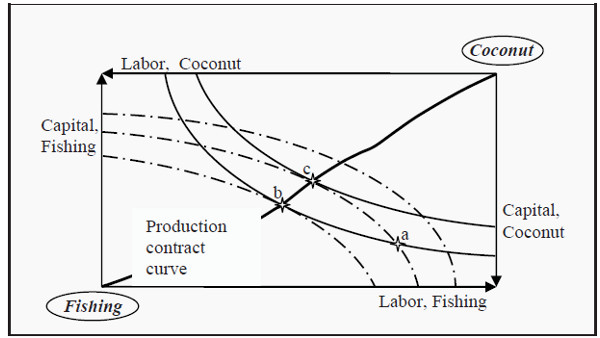
Figure 18.3: Edgeworth Box for Production
What is “wrong” with point a? The isoquant for fishing (the full line) has a slope that is smaller than the isoquant for coconuts (the broken line). In Production in the Long Run , we defined the marginal rate of technical substitution, MRTS, as the slope of an isoquant. Remember what MRTS means: If we use one unit less of labor, how much more capital must we use in order to produce the same quantity of goods?
The fact that the curves have different slopes implies that we can reduce the work in the fishing firm by a small amount and increase the capital in the same firm by a small amount to keep the quantity the same.
This will free up labor that we can put into the coconut firm instead while we have to reduce the capital employed in that firm by a small amount. However, since the isoquant for coconuts is steeper than the one for fishing, the change means that they can now increase the production of coconuts.
In Figure 18.3, we see that the criterion for having an efficient production is that the isoquant for fishing just barely touches the isoquant for coconuts. In such a point, the two curves have the same slope and the criterion can be expressed as
MRTS good 1 = MRTS good 2
If we, similarly to before, find all such efficient combinations of work and capital for the two goods and joint them into a curve, we get the production contract curve.
The Transformation Curve
In the last section, we derived the production contract curve. That curve is a collection of all efficient combinations of the two input factors. If we take those combinations, they also define how much we can maximally produce of one good, given a certain production of the other. Say, for instance, that we
produce 50 fish. What is the maximum number of coconuts that we are then able to produce? For us to achieve the maximum, we have to produce at an efficient point, i.e. at some point on the production contract curve. At some point on this curve, we produce 50 fish.
The maximum number of coconuts we are able to produce is then the number produced in that same point, say 100 coconuts. combinations of goods they each correspond to, and then use that information in a new graph, we can derive the so-called transformation curve (also called the production-possibility frontier).
The point from the example above, 50 fish and 100 coconuts will then be one point on the transformation curve. On the curve, we have all efficient production possibilities and underneath it, we have all other possible, but inefficient, production possibilities.
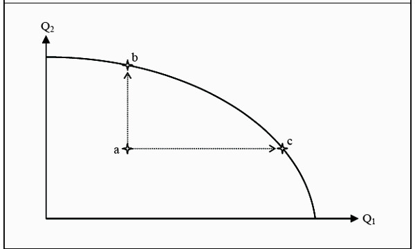
Figure 18.4: The Transformation Curve
The opportunity cost of producing one more unit of either good 1 or good 2? Since point a is not efficient, we do not have to give up anything to move to, for instance, point b. We just have to decrease the degree of waste in the economy.
Consequently, the opportunity cost is zero! However, when we have reached point b, we cannot increase the production of good 2 more without reducing the production of good 1. If we want to move from point b to point c, we, instead, have to give up a certain quantity of good 2 to compensate for the increase in good 1.
The quantity we have to give up is the opportunity cost. In other words, on the transformation curve the two goods have a price in terms of the other good, a relative price.
Note that the slope of the transformation curve is the same thing as what we in Baskets of Goods and the Budget Line defined as the marginal rate of transformation, MRT. To find MRT , we then used prices:
MRT = - p1 / p2
However, in the transformation curve there are no prices. Here, instead, we directly get the relative price of the goods.
However, note that this is what we got in Baskets of Goods and the Budget Line as well. The example we used there was that one ice cream costs 10 units (of the appropriate currency) and a pizza 20 units. If we insert those prices into the formula, keeping all units, we get
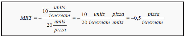
MRT is consequently the relative price for one good, expressed in units of the other good. Note that this means that the slope of the budget line in Baskets of Goods and the Budget Line is directly related to which point on the transformation curve one has chosen.
Pareto Optimal Welfare
We will now put production and consumption together in one diagram. We start from the transformation curve, and assume that society has come up with an efficient mix of goods 1 and 2, i.e. of coconuts and fish in our example.
The production will then lie on a point on the transformation curve, for instance, point a in Figure 18.5. The marginal rate of transformation, MRT , is the slope in point a, and we produce the quantity q1 of good 1 and q2 of good 2. Robinson and Friday now have to allocate the goods between themselves. We therefore add an Edgeworth box under the transformation curve, with one corner at point a and the opposite one at the origin.
An efficient allocation then requires that their respective relative valuations of the goods are equal, i.e. that MRSR = MRSF (where the subscripts refer to Robinson and Friday, respectively). In the figure, two such allocations are indicated: point b and point c, that both lie on the contract curve. (Also, compare to Figure 18.2.) We now have efficiency in production (since the total production is on the transformation curve) and efficiency in consumption (since the allocation is on the contract curve). Is that enough for us to have general efficiency?
No, it is not. It is also required that we produce what the consumers demand. There is one big difference between points b and c. In point b, the slope of the indifference curves, MRS, is the same as the slope of the transformation curve, MRT, in the point at which we have chosen to produce. That is not the case at point c. At point c, MRS is smaller in magnitude than MRT.
To see what the problem with that is, think of what MRS and MRT are. MRS is the price the consumer are willing to pay for one good in terms of the other, i.e. how many coconuts Robinson and Friday are willing to trade for one fish. Equilibrium in consumption demands that they have the same valuation. MRT, on the other hand, is the price the producers have to pay (given that the production is efficient) to produce one more unit of one good, again in terms of the other good.
If the consumers are willing to pay more for one good than they have to, there are unexploited opportunities and the situation cannot constitute a general equilibrium. If we change the production such that we produce more of the good of which the consumers have a high valuation, then at least one consumer will be better off without anyone else being worse off.
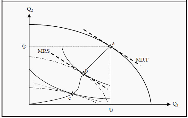
Figure 18.5: Pareto Optimal Welfare
The criterion for an efficient output mix is then that
MRS = MRT
A Definition of Pareto Optimal Welfare
We have now discussed three different types of efficiency:
- MRSR = MRSF; Efficient consumption. Robinson and Friday have the same marginal valuation of the goods. None of them can be made better off by a reallocation, without making the other one worse off.
- MRTS1 = MRTS2; Efficient production. The production of any of the goods cannot be increased without a reduction in the production of the other.
- MRS = MR; Efficient output mix. It will cost as much to change from one good to the other as the relative valuation. No consumer can be made better off by another output mix without making the other worse off.
If all these three criteria are fulfilled, we talk of Pareto optimal welfare
Externalities
In the remaining chapters, we will look at a few cases of market failures. A market failure is a situation in which the market fails to achieve an efficient allocation. A few such cases we have already seen. Both monopolies and oligopolies are, for instance, examples of market failures. In the following, we will briefly discuss externalities, public goods, and asymmetric information. Our consumption of goods does not occur in a social vacuum.
Much of our consumption, perhaps all of it, indirectly affects other people. The most classical example is pollution. It does not have to be a big factory; it could be your neighbors having a barbecue party. You do not participate, but you still get a share of the smell. You might take your car to work; you pay for the fuel but not for the pollution or the congestion to which you expose others. Other examples include the use of penicillin (you are cured, but contribute to making bacteria penicillin resistant), vaccinations, and a well-kept garden that your neighbors also enjoy looking at.
An externality is a situation in which the consumption or the production of goods has positive or negative effects on other people’s utility where these effects are not reflected in the price. It is common to distinguish between positive and negative externalities:
- Positive externalities. One person’s consumption of goods also increases other people’s utility without them having to pay for it.
- Negative externalities. One person’s consumption of a good decreases other people’s utility without them receiving any compensation.
Note that positive externalities are also a problem. Typically, we get too few goods with positive externalities and too many goods with negative externalities.
The Effect of a Negative Externality
Let us study the classical example of a negative externality: A firm produces a good, but in doing so they also pollute the environment. First, we need to define a few concepts:
- The marginal cost of the externality, ME. The change in the cost of the marginal effect, when production is increased by one unit. This is similar to the concept of MC, but instead of concerning the cost for the firm, it concerns the (uncompensated) cost of the externality.
- Social cost. The sum of the cost of producing the good and the cost of the external effect.
- Marginal social cost, MSC. The sum of the firm’s marginal cost and the marginal cost of the externality, i.e. MC + ME.
We can analyze this situation in a way that is similar to the one in Short-Run Equilibrium and Long-Run Production Look at Figure 19.1 (and compare, for instance, to Figure 9.2). The firm operates in a perfectly competitive market, so MR = p. To maximize its profit, the firm chooses to produce the quantity where MC = MR, i.e. the quantity qC.
However, this firm also emits pollution. The pollution does not cost the firm anything, but there is a cost to society. The more the firm produces, the more it pollutes. In the figure, we have drawn the marginal cost of the external effect, ME, and the marginal social cost, MSC = MC + ME. We see that for society, the optimal quantity to produce is qS.
The effect of the firm being able to ignore the cost of polluting is that it produces too much of the good. As an indirect effect of that, there will also be more pollution than at the optimum...
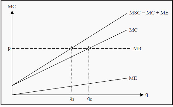
Figure 19.1: The Effect of a Negative Externality
Regulations of Markets with Externalities
One way to correct the situation in The Effect of a Negative Externality is to put a tax on each unit of the product. If one knows the size of ME then the tax should be that same amount. Thereby, the marginal cost curve of the firm will coincide with MSC, and the firm will automatically correct its production to the optimal quantity, qS. An obvious problem with this solution is that one rarely knows ME.
Other strategies to regulate the market include quantity regulations and the creation of transferable emissions permits.