Production and production costs
- Detalii
- Categorie: Microeconomics
- Accesări: 12,472
A producer uses raw materials, capital, and labor to produce goods and services. Here, we will present a simple model for how they decide how much to produce and which technology to use for production. A large part of producer theory is very similar to consumer theory.
Basic assumptions for consumer theory are that consumers have a goal to maximize their utility, but that they have restrictions due to limited income and prices. Producers also have a goal. They wish to maximize their profit. They also have restrictions. These are, for instance, the costs of labor and capital; but they also have restrictions regarding the technology of production.
An aspect that will also prove important for a firm is the amount of competition they face: Do they have one, a couple, or many competitors? Alternatively, do they not face any competition at all? We will study different market forms in later chapters.
- The producers have certain restrictions. Primarily because different combinations of inputs (labor and capital) have different associated costs.
- The firm operates in a market that, in turn, has certain structures that the firm cannot influence.
- Technology: Different combinations of input produce different quantities of goods.
- We will distinguish between production in the short run and in the long run. In the short run, the quantity of available capital is fixed; in the long run, both labor and capital are variable.
- Given production and restrictions, the producer maximizes her profit.
- Another important question is how large a firm should be. The important concept here is returns to scale. How firm size affects how efficiently it can transform input to output.
The Profit Function
We will use a very simple model of a firm. It produces a single good, and the most important input factors are labor and capital (for instance machines). The producer has a certain cost, C, and a certain revenue, R. Her profit, π, can then be written as the difference between revenue and cost:
π = R - C
The revenue, in turn, depends on the price of the good and how large quantity she sells,
R = p * q
The costs are, of course, also dependent on how large quantity she produces, but usually in a more complicated way. The profit can therefore be written as
π = p * q - C(q),
where C(q) means that the cost, C, is a function of the quantity, q.
We will analyze each of the three variables, p, q, and C, in the profit function. The price is often set by the market. C depends both on the costs of the input factors and the quantity produced. The firm therefore chooses the quantity that maximizes profit. In this chapter, we will analyze production. In section: Costs, we will look at the costs of production, and in later chapters, we will study different market forms.
The Production Function
The quantity the producer will produce of the single good, depends on the number of working hours, L (for Labor), and the amount of capital, K, that she uses. q is consequently a function of L and K:
q = f (L , K)
The letter f in the expression means that we have a function of L and K. That could mean 'L + K', 'L*K' or 'L2 + 9*ln(K)' to just mention a few arbitrary examples. Which function that is appropriate depends on the technology, which good one produces, etc.
Note that we, of course, assume that the production of q units is done in the most efficient way possible. If it, for instance, is possible to produce 10 units of the good using a certain combination of L and K, it is also possible to produce only 9 units with the same combination. However, that production cannot be efficient, since one is wasting resources that could be used for the production of one more unit.
Average and Marginal Product
Before we begin the analysis, we need to define a few concepts that will be important later on. The average product is how much of the good that on average is produced by a certain input, L or K. We therefore have that the average products, AP, for labor and capital, respectively, are
Average product: The quantity of goods that, on average, is produced per hour worked or per unit of capital.

The marginal product, MP, is how much extra quantity that can be produced if one increases the amount of either labor or capital with one unit, keeping the other one constant:
Marginal product: How much the quantity produced increses if either labor or capital is increased by one unit.

The expression for MP is, just as in the case of MRS, only approximate. It will also become more and more exact the smaller one chooses ΔK or ΔL.
The Law of Diminishing Marginal Returns
Beside the conclusion that "supply = demand", the law of diminishing marginal returns (or the law of diminishing marginal product) is probably the most frequently cited concept from microeconomics. Suppose we keep everything constant, except for one single input factor, for instance L. If we increase the number of hours worked, we will probably produce more. The law of diminishing marginal returns states that the increase will eventually become smaller and smaller when the number of hours worked is large enough.
To use an example: Suppose you start a firm that produces photocopies. You buy a powerful copying machine and you are the only worker. Say that you work one hour per day. You probably will not be able to make many copies during that time. The machine needs fifteen minutes to warm up, you need to prepare things, etc. If you increase the number of hours worked by one hour, you will probably make more copies during the second hour than during the first. Consequently, the marginal product is higher during the second hour than during the first, and over that interval, we therefore have increasing marginal product.
However, if you continue to increase the number of hours, you will eventually not produce many more copies per additional hour. You will become too tired to work. The same thing will happen if you hire other people to work for you: eventually, additional hours or additional workers produce very little additional output. If you, for instance, hire several people, the space will become crowded and the workers will become less efficient. This “law” is based on experience and speculation, but is not considered particularly controversial. We will use it when we construct the product curve.
Production in the Short Run
It is common to distinguish between the short run and the long run regarding production. The short run is defined as the time during which (at least) one of the input factors is fixed, usually capital. If the firm, for instance, buys a factory, it may not be able to increase or decrease its size as fast as they would wish. During the time that the firm is stuck with the factory as it is, it amounts to a fixed cost. In the long run, all costs are variable. We will assume that in the short run, labor is variable but capital is fixed. To make it clear that the quantity of capital is fixed in the short run, one often adds a line above the K in the production function: q = f (L, K).
The relationship between total production and the number of hours worked can be drawn in a graph. Often, one combines that graph with another graph that shows the marginal product and the average product of labor. We will now show how to construct such a graph.
The Product Curve in the Short Run
If we keep the amount of capital constant, the quantity produced is a just function of the number of hours worked, L. In Figure 7.1, we see a typical product curve with associated average and marginal product curves. The product curve has a few typical features: In the beginning, when the number of hours worked is low, production increases slowly, and later it becomes steeper and steeper. Eventually it reaches a maximum and thereafter it decreases.
After we have drawn the product curve, we want to construct the curves for the average and marginal product of labor. (The corresponding values for capital are not as interesting, since capital is a fixed cost in the short run.) To do that, we first observe that there is a simple method to find the value of the average product.
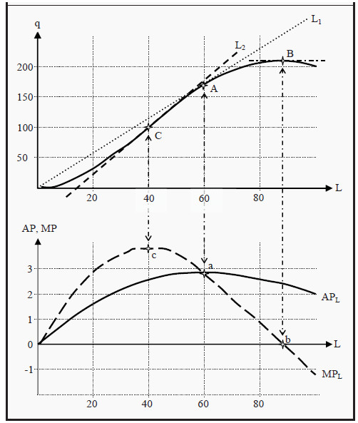
Figure 7.1: The Production Function with Average and Marginal Product
When you have drawn the product curve in the upper part of the graph, you draw a similar diagram below it with the same scale on the X-axis. Now, take a ruler and position it in the upper graph, with one point at the origin (0,0) and another at some point on the product curve, for instance as the line L1 indicated in the graph. The slope of the ruler will now be equivalent to the average product, APL, at that point where the ruler touches the product curve. (That is, APL at point A is equivalent to the slope of line L1.)
The maximum value of APL we get at point A, when L is 60. Indicate a point in the lower graph at L = 60, point a. To find the correct value on the Y-axis for point a, we calculate the slope of L1 in the upper part of the diagram: Point A is at L = 60 and q = 170, so the slope is 170/60 = 2.83. Point a should then be at (60,2.83) in the lower diagram. At point a, APL reaches its highest value and must consequently slope downwards both to the left and to the right. Draw such a curve and label it "APL.”
To construct MPL, let instead the ruler glide along the product curve in the upper graph so that it indicates the slope of the curve at different points. That way we can see that at point B, when production is at its maximum, the slope must be zero. Consequently, MPL = 0 in that point and we indicate the corresponding value for MPL in the lower graph, point b. Then, let the ruler glide along the product curve and note when the slope is as high as possible.
In Figure 7.1, that is at point C (when the ruler looks like L2). In that point, MPL reaches its highest value. Indicate it in the lower graph. It is easy from the upper graph to see that, in this case, the slope of L2 is higher than the slope of L1. Consequently, MPL (at point C) must be higher than APL (at point A) and point c in the lower graph must be higher than point a. After that, draw the graph for MPL: It must slope downwards both to the left and to the right of c. It must also pass through a (where MPL = APL) and then through point b. Now, the graph is finished. Note that we have obeyed the law of diminishing marginal returns: To the right in the graph, MPL becomes smaller and smaller (and eventually it becomes negative).
Note also that, the two graphs for MPL and APL in the lower graph are closely related to each other. MPL must intersect APL in the latter’s maximum point.
That fact has a purely mathematical reason: To the left of point a, MPL > APL. That means that when we add one more unit of L in that region, we produce exactly MPL more units of the good. Since that is more than the average so far, the average must increase. This is true as long as MPL > APL. To the right of point a, we have that MPL < APL. That means that if we add one more unit of L, we produce MPL more units of the good, which here is less than the average so far. Consequently, the average must decrease and APL must slope downwards.
Production in the Long Run
In the long run, both labor and capital are variable inputs. That means that the quantity produced is a function of both L and K, where either of them can be changed, i.e. q =f (L,K ) (and not f (L,(avg K). ).
It is usually the case that, the same quantity can be produced with a different combinations of labor and capital. Workers can, at least to some extent, be substituted for machines, and vice versa. This idea can be illustrated in a graph that is very similar to the indifference curves in consumer theory (see Section: Indifference Curves ).
An isoquant ("iso" = similar/same; "quant" = quantity) is a curve that shows different combinations of L and K that produce the same quantity of the single good (still assuming that the production is efficient). They are usually drawn in a way that is similar to indifference curves. Since we have diminishing marginal returns, they must slope less and less steep to the right. In Figure 7.2, you can see an example.
Start by looking at point A. With that combination of labor and capital (L1,K1), a maximum of q = 10 units of the good can be produced. The same quantity could also have been produced with the combination (L2,K2), point B. If one wants to increase the production to 23 units, one can choose, for instance, point C, where both the amount of capital and of labor has been increased.
Consequently, one can move from A to C only in the long run. In the short run, K is fixed. If one wants to increase production, one therefore has to choose the same K. If one wants to produce 23 units in the short run (assuming we start at point A), one has to choose the combination (L4,K1), point D, and if one wants to produce 41 units, one has to choose the combination (L5,K1), point E.
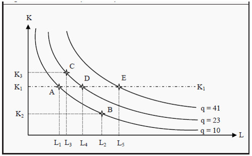
Figure 7.2: An Isoquant Map
Note that:
- Isoquants further away from the origin correspond to larger quantities.
- The isoquants cannot cross each other.
- The isoquants slope downwards.
- The extreme cases of isoquants are, just as for indifference curves, straight lines and L-shapes; compare to Figure 3.5.
The Marginal Rate of Technical Substitution
From the isoquants in the previous section, one can derive the marginal rate of technical substitution, MRTS. The MRTS corresponds to the marginal rate of substitution, MRS, from consumer theory (Section: The Marginal Rate of Substitution ).
The marginal rate of technical substitution: The amount of capital one has to add to production if one reduces labor with one unit but still wishes to produce the same quantity. Corresponds to the slope of the isoquant curve. MRTS can approximately be calculated as
MRTS= ΔK/ΔL
Since the curves slope downwards, if ΔK is positive then ΔL must be negative, and vice versa. That means that MRTS is a negative number. By convention, however, the minus sign is often omitted.
The Marginal Rate of Technical Substitution and the Marginal Products
There is an important relation between MRTS and the marginal products of labor and capital. As we have seen, MPL = Δq/ΔL, which means that if we increase the amount of hours worked with ΔL, production will increase with Δq = MPL * ΔL. Similarly, for capital we have that MPK = Δq/ΔK, so if we use one unit less of capital, production decreases with Δq = MPK * ΔK. For instance, if the marginal product of labor, MPL, is 3 and we add 1 more hour of labor, we will produce 3*1 = 3 units more of the good.
Let us combine these two observations in the following way: Suppose that you are on an isoquant, for instance in point B in Figure 7.2. If you increase labor with ΔL, production will increase with Δq = MPL * ΔL. However, suppose that you at the same time decrease your use of capital exactly so much that you still produce the same quantity as you did in point B. Then the total change in q must be zero. We can express this as

If we rearrange the last expression, we can get an alternative expression for MRTS (see the previous section):

The marginal rate of technical substitution, MRTS, which, by definition, equals (minus) the change in capital divided by the change in labor, also equals one marginal product divided by the other. Note that on the left-hand side, we have the marginal product of labor in the numerator but in the middle, we have ΔL in the denominator.
Returns to Scale
Suppose that, using labor L and capital K, we produce the quantity q of a good. If we would double both L and K, we would probably increase the quantity produced as well, but by how much? If q is also doubled, we have constant returns to scale (we can think of this as that the scale is the same for (L,K) and q). If instead q increases by less than two times, we have decreasing returns to scale, and if it increases by more we have increasing returns to scale.
More generally, we increase L and K by a factor t, and then check if q increases by more, less, or by the same factor. We can express this as
f( t*L, t*K ) < t*f (L, K) Decreasing returns to scale
f(t*L, t*K) = t*f (L, K) Constant returns to scale
f( t*L, t*K) > t*f (L, K) Increasing returns to scale
Look again at the expressions above: f(L,K) is the quantity produced from the start. We introduced this same expression in Section The Production Function. f(t*L,t*K) is the quantity produced if you increase both K and L by the factor t. Then you ask if you get more, less, or the same as t times the production you had from the beginning, i.e. t*f(L,K).
There can be different reasons why we get different returns to scale. For instance:
- Constant returns to scale. Suppose we have a factory that produces a certain quantity of a good. Then we build another factory that has the same size and that uses the same number of workers, so that we now have two factories. It seems reasonable to assume that the second factory produces the same quantity as the first one does. This means that, as we double the inputs we also double the output.
- Decreasing returns to scale. Suppose it becomes more and more difficult to coordinate the production as the size increases, so that we get higher and higher costs for administration. Then the costs will increase proportionally more than the production, and the production will grow by less than the inputs.
- Increasing returns to scale. Oftentimes, large firms are more efficient than small firms are. This is called large-scale advantages.
Costs
So far, we have only studied how different combinations of inputs produce different quantities of a good. Now, we will instead look at the cost of production. As before, we distinguish between the short and the long run. When we study costs, it is important that we use the opportunity cost as measure, i.e. the cost of using our resources equals how much they had been worth if we had instead used them for the best alternative. (See also Supply, Demand, and Market Equilibrium )
One reason for studying the cost side is that we want to find the cheapest way of producing a good. However, there is also another reason. The relationship between output and cost play an important role for which type of market that will arise: how many firms will there be, and how high the price will be relative to the cost of production. That question we will return to in later chapters.
Production Costs in the Short Run
In the short run, not all input factors are variable. We therefore distinguish between fixed cost, FC, and variable cost, VC. Total cost, TC, is the sum of the two:
TC = VC = FC
We also need to define a few other central concepts. Regarding average cost, we will have use for the averages of all three of the above. If we divide each of them with q, we get average total cost, ATC, average variable cost, AVC, and average fixed cost, AFC:

Note that the following must hold:
ATC = AVC + AFC
The marginal cost, MC, in turn, measures the cost of producing one more unit of the good:

Note that we can use either the change in total cost or the change in variable cost. Both must give the same answer, since the fixed cost does not change (ΔFC = 0). As before, the expression for marginal change is only an approximation.
Now, we will construct a graph to illustrate these different measures of costs (see Figure 8.1). The fixed cost, FC, is constant, independent of how many units we produce, so the curve illustrating FC must be a horizontal line. Total cost, TC, must always increase with production; else, the production is not efficient.
Furthermore, since if we produce nothing TC must equal FC, the curve for TC must start in the same point as FC on the Y-axis. Since TC = VC + FC, the curve for variable cost, VC, must have the same shape as TC. Obviously, VC of producing nothing is zero, so the curve for VC must start at the origin.
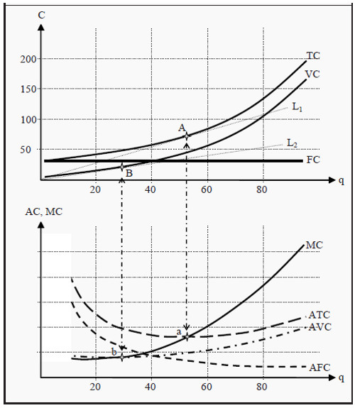
Figure 8.1: The Cost Function with Average and Marginal Costs
Using the curves we have drawn in the upper part of the figure, we will now construct the ones in the lower part, i.e. ATC, AVC, AFC, and MC. First, we use the same technique as we did in Section: The Product Curve in the Short Run. Lay a ruler in the upper part of the figure such that it has one point at the origin and another point on the TC curve. Find the point on TC where the ruler has the smallest slope. In the figure, this corresponds to line L1 and point A. You have now found the smallest possible average cost, ATC. Proceed in the same way to find the point on VC where the ruler has the smallest slope: the line L2 and point B. That point corresponds to the lowest possible average variable cost, AVC.
Draw the two curves for ATC and AVC in the lower part of the figure. Of course, ATC must lie above AVC. ATC should have its lowest point at a, and AVC at b. If you wish to find the numerical value for, for instance, point a, then read off the location of point A in the upper part of the figure: (53,75). Then calculate 75/53 = 1.4. Point a should then be at (53,1.4).
You can now also draw MC in the lower part of the figure. It must run through both point a and point b (for the same reasons as in Section: The Product Curve in the Short Run) and it should correspond to the slope of TC (or VC, since it has exactly the same slope) in the upper part of the figure. Note that, since the slope of TC becomes higher and higher, MC should increase as we move to the right. Lastly, AFC must become smaller and smaller the more products we produce, since FC is a constant and we divide with an increasingly higher quantity, q.
Production Cost in the Long Run
In the long run, both labor and capital are variable. That allows us to, in a way similar to the budget line in consumer theory, construct the so-calleds ("iso" = similar/same). If the price of one hour of work is w (for wage) and the price of one unit of capital is r (for rental rate), an isocost line is defined as all combinations of L and K that cost the same:
w * L + r *K =C
Solving this expression for K, we get

For the time being, we assume that the prices of labor and capital are given. If we insert a few different values for C, we can draw a few isocost lines, for instance the lines C1, C2, and C3 in Figure 8.2. Similar to the budget line, the slope of the isocost line depends on the value of w/r, and the easiest way to draw the budget line is to find the points on the X- and Y-axes where one buys only labor or capital. One can, for instance, calculate C1/r, indicate that value on the Y-axis, and C1/w, and indicate that value on the X-axis. Then draw a straight line between the two points to get all combinations of L and K that cost C1.
Now, you can probably see where we are heading. In Figure 8.2 we have also drawn an isoquant, and in point A, the isoquant just barely touches one of the isocost lines, C2. If we are prepared to pay the cost C2, then q = 23 is the maximum quantity we can possibly produce. We do that by choosing the quantities L* and K* of labor and capital, respectively.
Note that we can also reason the other way around. If we want to produce 23 units, then the lowest cost we can possibly do that at is C2. The optimal choices of inputs are then L* and K*. For a production of exactly 23 units of the good, all other combinations of L and K are either inefficient or do not produce enough of the good.
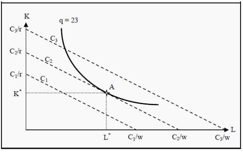
Figure 8.2: Isocost Lines
Just as we did in consumer theory, we can give a mathematical formulation of the result. At the point of tangency, the isoquant and the isocost line must have the same slope. The slope of the isocost line is -w/r and the slope of the isoquant is the marginal rate of technical substitution, MRTS . At the point of tangency, we must then have that

Note that, if one uses the convention to omit the minus sign in front of MRTS, one must also do so in front of w/r. As a reminder, we have also included how we found MRTS earlier. It is important to understand how to interpret this criterion. If we rearrange the expression, we can get

Remember that MPK is the number of additional units we produce if we add one more unit of capital, while holding everything else constant. MPL is the same for one more unit of labor. MPK/r is then the number of additional units we get per dollar (or other currency), if we use one more unit of capital. MPL/w is the number of additional units we get per dollar if we use one more unit of labor (work one more hour). At the optimal point, these two must be equal, and the producer is then indifferent between using labor and using capital.
If we repeat the procedure for finding the optimal point for many different isocost lines and isoquants, we will trace out a curve that shows all efficient combinations of labor and capital. This is the so-called expansion path. From that curve, it is possible to derive the long-run cost of production. (Compare to the income-consumption curve and the Engel curve in Section: The Engel Curve ) Look at Figure 8.3. In the upper part of the figure, we have drawn three isocost lines, C1, C2, and C3, and then found the points on each of them where an isoquant just about touches them. The three points are A, B, and C where the produced quantities are 100, 300, and 500 units of the good. If we had done this for all possible costs, we would have gotten the long-run expansion path. We
see that, for a cost of C1 we can produce a maximum of 100 units, for C2 a maximum of 300 units, and for C3 a maximum of 500 units. In the lower part of the figure, we have indicated those combinations at points D, E, and F, and then drawn a line through them. That line is the long-run cost of production. Note that the line must start at the origin, since the long-run cost of producing nothing is zero.
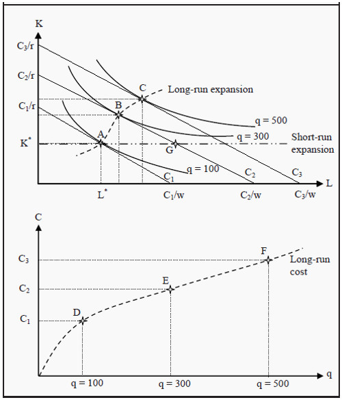
Figure 8.3: Derivation of the Long-Run Cost Curve and the Expansion Path
In Figure 8.3, we have also drawn the short run expansion path. In the short run, the quantity of capital is fixed, K*. In the diagram, that amount of capital is optimal for a production of 100 units. That can be seen from the fact that the isocost line C1 touches the isoquant q = 100 in point A where the amount of capital is K*. If we want to produce more than 100 units in the short run, we
must do that using only additional labor, i.e. the expansion must follow the short-run expansion path. At point G, the cost of production is as high as at point B, but the number of produced units must be smaller since the isoquant q = 300 is further from the origin than point G. When one chooses the long-run amount of capital to use, one does so under the assumption that the production in the short run will be optimal at precisely that amount. In the diagram, one has chosen K* because one believed that, in the short run one will produce 100 units. For other quantities, K* is not an efficient choice.
The Relation between Long-Run and Short-Run Average Costs
As we saw above, the short-run cost of production must always be higher than the long-run cost, except for at one certain point where they are the same. In Figure 8.3 the short-run cost and the long-run cost of producing 100 units is the same, given that one has chosen an amount of capital equal to K*. For every other choice of capital, it is more expensive to produce 100 units in the short run than in the long run.
If this is true about the cost, it must also be true about the average cost, i.e. the long-run average cost must always be smaller than the short-run average cost, except for at one point where they are the same. If we draw a few different curves for short-run average costs, where each curve is valid for different longrun investments in capital, we get a picture as the one in Figure 8.4.
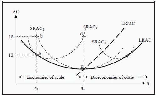
Figure 8.4: Long-Run and Short-Run Average Costs
We have three different short-run average cost curves, SRAC1, SRAC2, and SRAC3 (Short Run Average Cost) and one long-run average cost curve, LRAC (Long Run Average Cost). Each SRAC curve has one point where it is optimal in the long run as well. For example, SRAC1 is optimal at point a, where it touches LRAC and the average cost is 12. If one had instead chosen a different amount of capital, for instance, such that one would have been constrained to SRAC2, one would have ended up at point b if one wanted to produce the quantity q1. Average cost would then have been 18. SRAC2 is instead long-run optimal if one wants to produce q2.
If one takes all such points where the short-run average cost is optimal, i.e. for all possible SRAC curves, not just the ones drawn here, one will get the curve for the long-run average cost, LRAC. Just as the short-run marginal cost curves must intersect the SRAC curves at their lowest points, the long-run marginal cost curve, LRMC, must intersect LRAC at its lowest point.
The LRAC curve in Figure 8.4 has another interesting property. To the left of the quantity q2, LRAC slopes downwards (towards q2), but to the right it slopes upwards. That means that the lowest cost per unit of the good is achieved at the quantity q2 and at point c in the diagram. To the left of q2, we have economies of scale and to the right we have diseconomies of scale. Note that this can be very important if there is competition in the market. If the firm is at a point to the left of q2, it can lower its cost per unit by increasing the scale of production. In the next step, it can undercut the price of its competitors.