Supply, Demand, and Market Equilibrium
- Details
- Category: Microeconomics
- Hits: 7,465
We begin our study of microeconomics by looking at a market with many buyers and sellers, i.e. a market where there is a large amount of competition. We will study such a market in more depth in Perfect Competition, as well as other market types, but starting here makes it easy to get a feel for how the subject works.
Demand
The Demand Curve
The demand curve shows what quantities of a good buyers are willing to buy at different prices. Note the expression “are willing.” It is not about how much they actually buy, but about how much they would want to buy if a certain price was offered. A demand curve is only valid if all other relevant factors are held constant (ceteris paribus: with other things the same). The most important other factors that can affect demand are:
The buyers’ income.
Prices and price changes on other goods. We will make a distinction between complementary goods and substitute goods. An example of complementary goods is right and left shoes. If the price of right shoes rises then the demand for right shoes will typically decrease. However, the demand for left shoes will also typically decrease. Consequently, the demand for left shoes partly depends on the price of another good: right shoes.
Substitute goods work in the opposite way. An example could be blue and green pens: If one cannot use blue, one can often use green instead. If the price of green pens rises, the demand for green pens typically decreases. However, if the price of blue pens is unchanged one can use these instead of the green ones, and then the demand for blue pens increases. Consequently, the demand for blue pens depends on the price of another good: green pens.
Note that for substitute goods, a rise in the price of the other good leads to an increase in the demand for the good we are analyzing, whereas for complementary goods it is the other way around; a rise in the price of the other good leads to a decrease in the demand for the good analyzed.
Preferences. What consumers demand is largely a matter of taste. If there is a change in taste, there is usually also a change in demand. Taste can change for many different, underlying, reasons. For example, changes in moral perception or in fashion.
If these factors are held constant, then the demand curve is valid and it usually slopes downwards. In other words, the lower the price is the higher is the demand, and vice versa. Demand is defined for a certain period. One can for example think of it as defined over a month, corresponding to a monthly salary.
When drawing a demand curve in a diagram, the quantity demanded is on the X-axis and the price is on the Y-axis. This is slightly odd, since we often think of the quantity demanded as a function of the price, not the other way around. There are historical reasons for drawing it this way.
When do We Move along the Demand Curve, and When Does It Shift?
The relation between price and quantity that is described by the demand curve is valid only if it is the price of the good itself that changes. Look at Figure 2.1 and the demand curve D1. If, in the beginning, the price is p1, then the quantity demanded is Q1 (point A). If the price of the good falls to p2, then the quantity demanded changes to Q2 (point B). We, consequently, move along the demand curve when the price of the good changes.
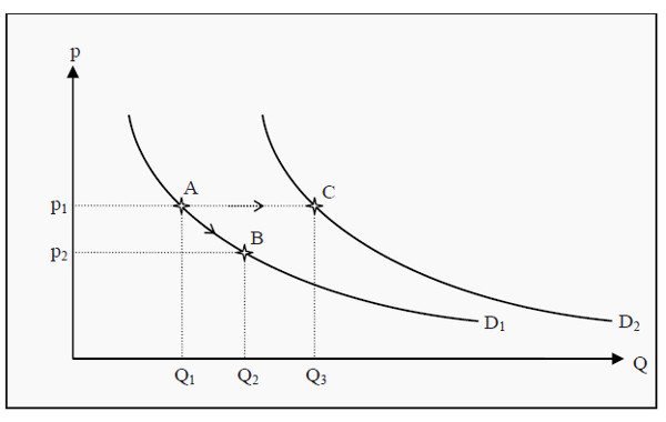
Figure 2.1: The Demand Curve
If, instead, something else changes (e.g. income, the prices of other goods,consumer preferences, or anything that affects the demand on the good), then the demand curve shifts. Assume again that the price is p1 so that the quantity demanded is Q1 (point A). If the consumer’s income increases, she can buy more of the good than she could before. Consequently, the whole demand curve shifts from D1 to D2. If the price is still p1, the quantity demanded increases to Q3 (point C).
Supply
The Supply Curve
The producer counterpart to the demand curve is the supply curve. It shows how large quantities the producers are willing to sell at different prices, given that other factors that can affects supply are held constant. The supply curve is typically upward sloping or horizontal (but it could also be downward sloping see more The Law of Supply).
The demand curve is also valid over a certain period. Later, we will distinguish between two time periods: short and long horizons. The most important factors, besides the price, that affect supply are:
- Factor prices, i.e. wages, prices of machines and compensation to owners and lenders. In other words, changes in the cost of production.
- Laws and regulations that apply to the production.
- Prices of other goods the firm produces or could potentially produce. Perhaps the producer is producing blue and green pens. If the price of green pens rises, she is likely to shift over resources (workers and machines) to that production and there is less left with which to produce blue pens. Consequently, the supply of blue pens decreases, even though the price of blue pens is unchanged.
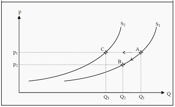
Figure 2.2: The Supply Curve
The supply curve behaves in a way that is similar to that of the demand curve. Look at Figure 2.2 and the supply curve S1. If the price is p1, then the producers are willing to sell the quantity Q1 (point A). If the price of the good falls to p2, we move along S1 to point B, where the quantity is Q2. If, instead, some other factor changes, e.g. if wages increase so that it becomes more expensive to produce the good, the whole supply curve shifts. For instance from S1 to S2. If the price is still p1, then the quantity supplied changes from Q1 to Q3 (point C).
Equilibrium
A market is in equilibrium when both of these conditions are fulfilled:
- No agent wants to change her decision or strategy.
- The decisions of all agents are compatible with each other so that they can all be carried out simultaneously.
If we join the supply and demand curves in one diagram, we get an equilibrium point where the two curves intersect. At this point, the price the consumers are willing to pay is the same as the price the producers demand. In Figure 2.3, the equilibrium price (market-clearing price) is p* and the equilibrium quantity is Q*.
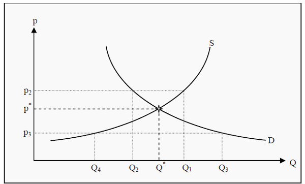
Figure 2.3: Equilibrium
The equilibrium point has two important properties in that it is most often (but not always) stable and self-correcting. That it is stable means that, if the market is in equilibrium there is no tendency to move away from it. That it is self-correcting means that, if the market is not in equilibrium then there is a tendency to move towards it.
To see more clearly what this means, suppose the price is higher than in equilibrium, e.g. that it is p2. At that price, producers are willing to supply the quantity Q1 whereas the consumers are only willing to buy the quantity Q2. Therefore, there is an excess supply of the good. To get rid of the extra units the producers are prepared to lower the price. This will push the price downwards, closer to p*. At p*, there is no excess supply and the downward push on the price ends.
Then assume, instead, that the price is lower than p*, e.g. that it is p3. At this price, the consumers demand quantity Q3 whereas the producers are only willing to supply the quantity Q4. Consequently, there will be a shortage of good, and the consumers will be prepared to bid up the price to get more units.
This will tend to push the price upwards, closer to p* where, again, the push will end.
How to Find the Equilibrium Point Mathematically
Supply and demand can be written as mathematical functions, and in simple examples, they are often straight lines. They could, for instance, be:

Here, QD is the quantity demanded, QS is the quantity supplied, and p is the price. We now want to find the price, p*, that makes QD = QS. If the left-hand sides above are equal, the right-hand sides must also be so. Therefore, substitute p* for p and set the right-hand sides equal to each other:
85+ 30p* + 185+ 20p*
To get p* alone on the left-hand side, we add 20 p* on both sides and subtract 85 from both sides. Then we have that
50p* =100.
Dividing by 50 on both sides yields the result that
p* = 2
If we then want to know the equilibrium quantity, Q*, we substitute the result we got for p* into either the supply or the demand function above. (Note that they must yield the same quantity, since p*, by definition, is the price that makes QD = QS.)
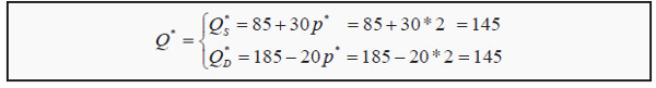
Consequently, we have the equilibrium price, p* = 2, and the equilibrium quantity, Q* = 145.
Price and Quantity Regulations
Many markets are, for a number of reasons, regulated. The government could for instance decide about prices that the market is not allowed to go above or below, or about maximum quantities. Such regulations will benefit certain groups of people, but often have unintended negative side effects. These are often called secondary effects.
Minimum Prices
Minimum prices (also called price floors) are often used for wages (the price of labor) and for certain types of goods such as agricultural goods. The minimum price is usually chosen above the equilibrium price, as in the opposite case it would not have any effect. (The market participants would then choose p* instead.) Consumers and producers are consequently prevented from reaching the equilibrium price p*.
Look at Figure 2.4. The effect of the minimum price is that the consumers only demand the quantity Q2 whereas the producers supply the quantity Q1. Therefore, we get an excess supply of the good.
Note that consumers and producers are allowed to buy and sell at any price above the minimum price. A price higher then pmin will however result in an even larger excess supply, so typically the minimum price is chosen.
The situation described is not an equilibrium. To see that, note that point 2 in the definition of equilibrium is not satisfied: Given the price pmin producers want to sell the quantity Q1, but that is not possible since the consumers only want to buy the quantity Q2.
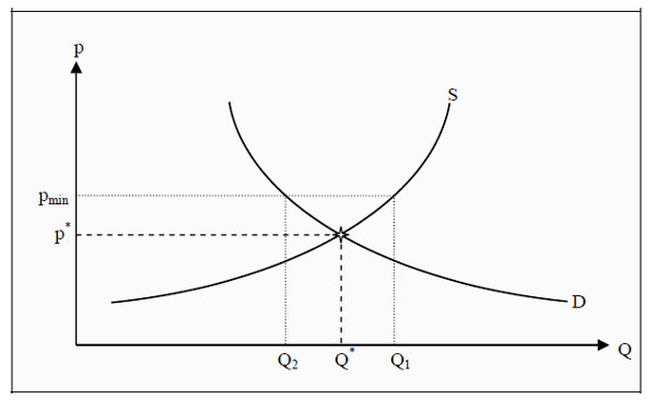
Figure 2.4: The Effect of a Minimum Price
Maximum Prices
Maximum prices (also called price ceilings) are in several countries used for apartment rentals. For a maximum price to have any effect, it has to be below the equilibrium price, and the effects are the opposite to those of a minimum price. In Figure 2.5, pmax is the maximum price. It causes the consumers to demand
the quantity Q1 whereas the producers only want to supply Q2, and, consequently, there is a shortage. A typical consequence of a maximum price is that the search time to find an appropriate good is increased since the supply is too small to meet the demand.
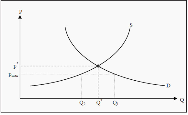
Figure 2.5: The Effect of a Maximum Price
Quantity Regulations
The effects of quantity regulations are similar to those of price regulations. Assume for instance that there is a restriction stating that one may only import the quantity Qmax of a certain good, say Asian textiles.
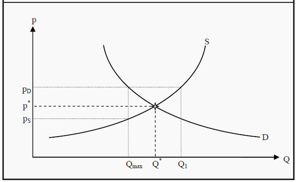
Figure 2.6: The Effect of a Quantity Regulation
Producers would have been willing to supply the quantity Qmax at a price of pS, whereas the consumers would have been willing to buy that quantity at a price of pD. Since the quantity is not allowed to increase, there is excess demand at all prices other than pD. When there is excess demand, consumers are likely to bid up the price, so the price that this market is likely to arrive at is pD. Note that at the price pD, producers are willing to supply a much larger quantity, Q1, but that they are prevented from doing so by the regulation. The consumers
have to pay a price that is larger than the equilibrium price (pD instead of p*) and they get fewer units of the good, so they typically are made worse off by a quantity regulation.