The complete Keynesian model
- Detalii
- Categorie: Macroeconomics
- Accesări: 15,892
Wage inflation
In this article, we will continue to develop the Keynesian model removing the assumption of fixed nominal wages. We define wage inflation πw as the percentage average increase in wages. Wages and wage inflation are still exogenous, i.e. they are not determined within the model. One justification for this assumption is that wages often are determined by agreements which often last for several years.
We do not need a new model to deal with inflation. Non-constant wages can be handled within all three Keynesian models as long as they are exogenous. The reason we chose to let wages be constant in the previous Keynesian models were entirely pedagogical – these models are easier to understand when wages are constant.
Price Inflation
The main reason for allowing for non-constant wages in the model is that we then can allow for persistent inflation/deflation. With constant wages, we cannot have persistent inflation as real wages would go to zero.
Neutral inflation is defined as a situation where wage inflation is equal to inflation (in prices). With neutral inflation, the real wages are constant. The Keynesian model does not require neutral inflation and real wages may vary over time. However, we cannot have an inflation which is always greater than or always smaller than wage inflation as real wages again would go to zero or infinity (again, remember that growth has been removed so we expect no upward trend in real wages). However, a few adjustments must be made in the models when we have inflation.
Adjustments to the Keynesian models when wages are no longer constant
Real interest rates, nominal interest rate and expected inflation
When we have inflation, we cannot, of course, assume that expected inflation is zero. Therefore, real interest rate will no longer be equal to the nominal interest rate and we must use:
R = r + πe
In this article, expected inflation πe is exogenous (although not necessarily constant. In more advanced Keynesian models you will find various assumptions on how expectations are formed.
Aggregate demand with inflation
In previous versions of the Keynesian model, none of the components of aggregate demand depended on P. In the IS-LM and in the AS-AD models, investments depended on the nominal interest rate R. We argued that investment actually depends on the real interest rate r, but since R = r when πe = 0, we could make it a function of R. When πe no longer is zero and the real interest rate r = R − πe, we should write:
I(r) or I(R − πe)
We should also write YD(Y, r) or YD(Y, R − πe). Since inflation expectations are exogenous (given), it is still the case that YD depends negatively on R. Note that if there is an equal increase in expected inflation and in nominal interest rate, real interest rate is unaffected and so is investments and aggregate demand.
The IS curve with inflation
We can draw the IS curve for a given value of πe. As previously explained, the IS curve is not affected by changes in P. However, it will shift upwards when πe increases.
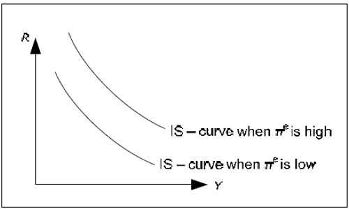
Fig. 14.1: The IS curve and expected inflation.
If πe increases, R must increase by the same amount to keep r and YD unaltered.
The money market with inflation
Let us begin with the money market diagram in 12.3.6 and introduce inflation. Since the MD depends positively on P, the MD curve to “glide” out towards the right when inflation is positive and toward the left when we have deflation.
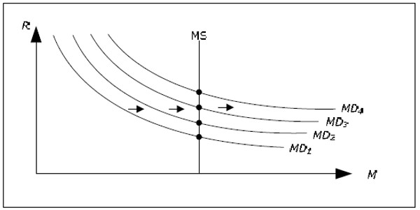
Fig. 14.2: The money market with inflation and constant money supply.
If money supply is constant, nominal interest rate will continuously increase when we have inflation and continuously decrease when we have deflation.
An interesting special case is when money supply increases by the same rate as P. In this case, the money supply curve will also glide outwards or inwards (depending on whether we have inflation or deflation) at exactly the same rate as the money demand. The nominal interest rate will then be constant.
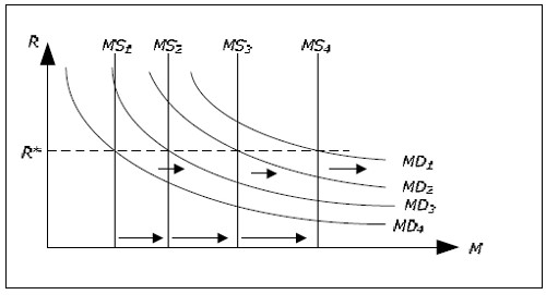
Fig. 14.3: The money market with inflation and rising money supply.
If we let πM denote the growth rate in money supply, we can conclude the following. For a given Y, R will increase if π > π M (prices increase faster than the money supply) and R will fall if πM > π. R isunchanged if π = πM. For example, when π > πM, the MD curve glides out to the right faster than MS curve which is why R increases.
The LM curve with inflation
In the previous article we found that the LM curve will shift upwards when P increases (assuming MS is constant). This is still true but we can also add that the LM curve glides upwards if π > πM (as R increases) and the LM curve glides downwards if πM > π.
The previous result is a special case of this result. If P increases, then π > 0 and if MS is constant then πM = 0 and the LM curve glides upwards. Earlier, we only considered cases when P jumped (from say 100 to 120). This translates into having inflation for a short period, an LM curve that glides upwards and when P reaches 120, inflation cease and the LM curve will stop moving.
The IS-LM model with inflation
The basic assumption
In IS-LM-model, we developed the IS-LM model with constant wages and prices. We can now extend this model to allow for inflation. Instead of constant wages and prices, we must assume that π = πW = πe. In the same that we dropped the assumption of constant P when we went on to the AS-AD model to allow for changes in real wages, we will drop the assumption that π = πW in section Inflation to allow for inflation and changing real wages.
Let us briefly justify the assumption π = πW = πe. πW = πe may be explained by realizing that if workers expect 6% inflation, they will demand 6% wage increases to maintain the same real wage (they usually require more than 6% and an increase in real wages, but this is because the growth of the economy will allow for this – always think of these models as if there is no growth).
The assumption π = πW means that we have a balanced inflation. As in the IS-LM model, the real wage is then constant. This is a reasonable assumption if the economy is in a state where aggregate demand is insufficient and L is lower than the profit-maximizing level.
Results
If πM = π and πe = π , both the IS- and the LM-curve will be fixed.
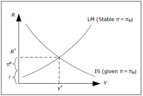
Fig. 14.4: The money market with inflation and constant money supply growth.
It is then possible to determine R* and Y * exactly as we did in IS-LM-model. We can also determine the real interest rate as r = R − πe and πe is given. All variables are now determined. Since π and πW are exogenous, P and W are given over time (as long as we know P and W at one point in time). L is determined exactly as IS-LM-model and we do not allow L to exceed LOPT as this would require a drop in real wages π > πW at least for a while.
If, for example πM < π, the LM curve will glide upwards, R (and r) will increase while Y will fall. In a model with inflation, we typically consider changes in the growth of the money supply, πM, rather than changes in the in the money supply itself when we discuss monetary policy.
The AS-AD model with inflation
In AS-AD model we removed the assumption of constant prices to allow varying real wages. The resulting model was called the AS-AD model. In the same way, we now remove the assumption that π = πW (but remember the discussion in 14.1.2 – π may only deviate from πW temporarily and they must be equal on the average).
The AD-curve at a given point in time
The AD-curve, just like before, displays combinations of P and Y where both the money market and the goods market are in equilibrium. At any given time, even when we have inflation, aggregate demand will as before depend negatively on P. The explanation, as follows, is little more involved.
Say that the price level one year ago was 100 and that P is the price level today. Then π = (P − 100)/100 is the rate of inflation during the previous year and P = (1 + π)*100 today. For example, if π is 10%, we have P = (1 + 0.1)*100 = 110 today. Given the price level in the previous year, we have a positive relationship between P and π.
Given price level last year, there is a price level today which would make inflation exactly the same as the growth rate in money supply over the last year. For example, say that πM was 4% in the previous year and P was 100 a year ago, then if P = 104 today we have π = π M, the IS- and LM-curves are stable and we can find the level of GDP which gives the equilibrium in both markets by finding thepoint where they intersect.
Now, to show that the AD curve slopes downwards, we must show that if P > 104, a lower level of GDP will result in simultaneous equilibrium. To see this, simply note that for P > 104, the inflation has been a little higher and the LM curve will be a little higher up resulting in a lower level of GDP. A similar argument shows that GDP must be higher if P < 104 for both markets to remain in equilibrium.
Thus, at a given point in time, given the price level last year, aggregate demand will still depend negatively on P and the AD curve will slope downwards.
The AD curve over time
With inflation, the AD curve will no longer be stable over time. Instead, it will glide upwards or downwards at a rate determined by the growth rate of the money supply πM. Let us look at the case πM = 10%.
If AD1 is AD curve in year 1, AD1 will show us all combinations of P and Y where both markets are in equilibrium in year 1. For example, both markets are equilibrium at point A where P = 100 and Y = 10.
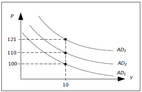
Fig. 14.5: AD curve glides if πM ≠ 0.
In year 2, the money supply is higher – it has increased by just 10%. If P had increased by 10%, thenthis new value of P together with the level of GDP we had last year would still give us equilibrium in both markets. Inflation has then been 10% and none of the IS or LM curves have shifted.
In year 2, P = 110 and Y = 10 must be on AD2. In year 3, by the same arguments, P = 110*1.1 = 121 and Y = 10 must be on the AD3 and we see that the AD curve glides upwards by 10% per year – exactly the same rate as the growth in the money supply.
We must remember that if πM ≠ 0, then the AD curve is applicable only for a given point in time. At another point in time, we must draw a different AD-curve. The rate at which the AD curve glides is equal to πM – if πM is high, a higher inflation is necessary if the same level of GDP is to lead to equilibrium in both markets.
Even though πM determines the evolution of the AD curve over time, there are still many combinations of P and Y leading to equilibrium in the goods- and money market (all points on the AD curve at precisely the given point in time). Only one point will be an equilibrium point for the entire economy and, as before, the AS curve will help us to find this point.
The Labor Market
Remember the model of labor market in the AS-AD model with constant wages. On the y-axis, we had real wage and on the x-axis, we had L (see Figure 13.6). The response curve had two parts, a horizontal part and a downward sloping part. On the horizontal part, prices where constant and L was determined by the aggregate demand.
Real wages in this part of the response curve may be denoted by (W/P)MAX as real wages can never be higher than this level. On the downward sloping part of the response curve, P is no longer constant and L is determined by P. On this part of the curve, the real wage is lower than ( W/P)MAX. We also concluded that the real response curve is a smooth version of this one.
With inflation, the reaction curve will not change. The reason for this is that we have real wages on the y-axis. If wages increase by 10% while prices increase by 10%, real wage will not change. In our model of the labor market with inflation, there is still a maximum real wage ( W/P)MAX. As longas we are to the left of point B, there is no reason for firms to change the growth rate of prices (which is given by π = πW) and the real wage will remain constant. In order to induce firms to go past the LB, real wages must fall below (W/P )MAX which means that prices must increase faster than wages: π > πW.
However, we must be careful with the notation:
- With no inflation, we said that said prices were constant on the horizontal part. With inflation, we must say that we have neutral inflation (π = πw) on the horizontal part.
- With no inflation, we said prices increase as L increase on the downward sloping part. With inflation, we must say that prices increase faster than wages as L increase on this part.
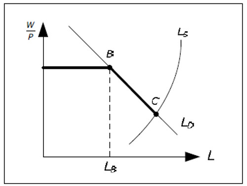
Fig. 14.6: The labor market with inflation.
The AS curve
Say that the nominal wage in year 1 (at a particular point in time) is equal to 1000. On the horizontal part of the response curve, real wage is constant and equal to its maximum value. Say that (W/P)MAX = 10. On the horizontal part, P1 = 100, where P1 is the price level in year 1. Firms will employ at most LB at this real wage. For firms to hire more than LB, P1 must be higher than 10. We realize that the AS curve at this point in time, AS1, will look like before. First, it is horizontal along P = 10, then, for higher Y. it is upward sloping.
Suppose that πW is equal to 10%. Next year, nominal wages will be equal to 1100. Wages in year 2 are determined by πW which is an exogenous variable, making wages in year 2 exogenous. As the maximum real wage is given and equal to 10, we conclude that P2 is equal 110 on the horizontal part of the response curve and that P2 > 110 on the downward sloping part. AS2 glides upwards up by 10% as given by the wages inflation. Using the same argument, P3 = 121 on the horizontal part of the response curve at year 3 and so on.
Just like the AD curve, the AS curve is to glide upwards or downwards depending on whether πw > 0 or πw < 0 when we allow for inflation. As for the AD curve, the AS curve is applicable only at a particular point in time if πW ≠ 0. At another point in time, we must draw a new AS curve.
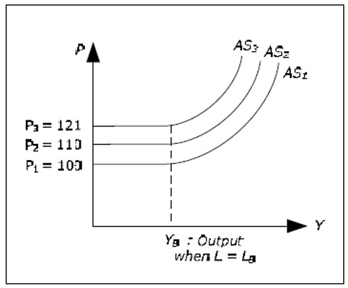
Fig. 14.7: AS curve gliding if πW ≠ 0.
The AS-AD model with inflation
When we have inflation, both the AD curve and the AS curve will be gliding. “The glide rate” of the AD curve is given by πM while it is π W which applies to the AS curve (where both rates are exogenous). Using the AS-AD curves, we can determine the equilibrium price P (and thus π) at any point in time and we can determine all endogenous variables. For example, we realize that if πM = πw, both curves glide at exactly the same rate. Y will then be unchanged and π will be equal to πw.
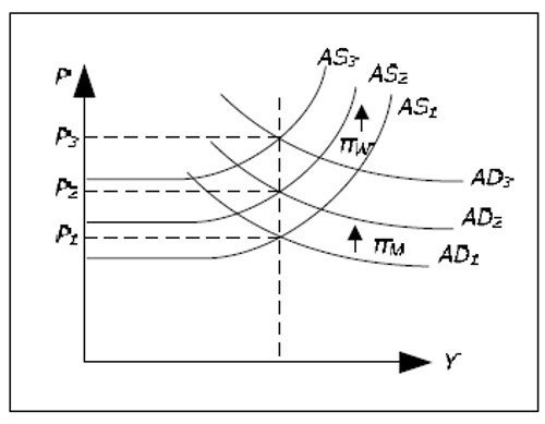
Fig. 14.8: Determination of Y and P in the AS-AD model with inflation.
The Phillips curve
The problem with the Keynesian model
We can identify two problems with the Keynesian model as developed so far:
- πW is exogenous. Even though inflation may temporarily deviate from the wage inflation, this deviation cannot be too large and it cannot last for too long (as real wages would becomeunreasonable low or unreasonable high). This model has no determination of πW and therefore no complete determination of π. A model that predicts an inflation of around 6% by assuming a wage inflation of 6% is not very useful. The Keynesian model with inflation is thereforeincomplete.
- It is quite unreasonable to assume that πW would be independent of Y. More reasonable would be to model πW as a positive function of Y. If we are in a boom, L will be above its averageand unemployment below its average. In such a situation, it is reasonable to expect wage inflation to increase.
To solve these problems, we need to make πw endogenous. We do this by to the Keynesian model adding the Phillips curve.
The Phillips curve
According to the traditional Phillips curve, there is a negative and stable relationship between wage inflation and unemployment.
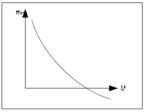
Fig. 14.9: The Phillips curve.
The Phillips curve is often drawn with π instead of πW on the y-axis, but since these variables may deviate only temporarily, the difference is small. The Keynesian model plus the Phillips curve provides us with a full determination of all variables.
Some comments on the Phillips curve
- The Phillips curve was initially an empirical relationship between wage inflation and unemployment that was observed in many countries. It was usurped rather quickly and many Keynesian economists and integrated into the theory because it allowed them to determine inflation within the model.
- The Phillips curve was not a part of Keynes original theory. The relationship was discovered long after Keynes wrote the "General theory". Therefore, many prefer to view the Phillips curve as an addition to the Keynesian model – not as a part of the Keynesian model.
- The Phillips curve is often interpreted as an important political curve. Some view this curve as giving the government a choice of low inflation or low unemployment (or something in between). Most economists, however, do not share this view – the reason for tis will be explained in the next article
- The Phillips curve can also be interpreted in the terms of the business cycle. In a boom, Y is high; U is low and π is high. In a recession, the opposite holds. In a boom, we are at a point up on the left on the Phillips curve, while in a recession, we are at the bottom right. Business cycles may be viewed as oscillations between these two points.
Determination of all endogenous variables
We can illustrate how all the endogenous variables are determined in the following diagram:
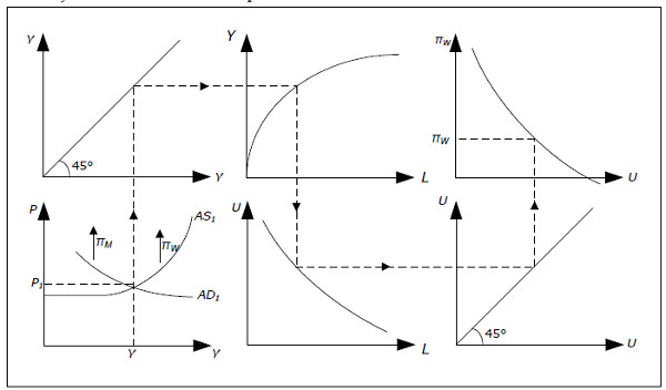
Fig. 14.10: The Keynesian model with the Phillips curve.
- Start at the bottom left. In year 1, AD1 and AS1 apply, the price level is P1 and GDP is Y.
- Extend this level of GDP up to the top left diagram and through the 45-degree line to the production function at the top in the middle.
- In this diagram we can determine how much L we need to produce Y. Extend this amount of labor down to the lower middle graph and through the 45-degree line to the bottom rightgraph.
- This diagram shows the relationship between L and U. The higher the unemployment rate U, the lower the amount of labor L and the curve slopes downwards. From L we can determine U which we extend up to the Phillips curve in the right top graph.
- From the Phillips curve, we can determine wage inflation πW.
- Going back to the AS-AD diagram, we now the rate at which the AS curve slides up or down.
The AD curve slides at a rate determined by πM which is exogenous.
An important case is when the growth in money supply is equal to the wage inflation. In this case, Y is fixed and π = π w = πM. If, however, πM exceeds the wage inflation, the AD curve will glide upwards at a faster rate than the AS curve. Now Y will increase and if you follow the effect through all the 6 diagrams, you see that L will increase, U will decrease and πW will increase. Y will continue to increase as long as πW< πM which means that W will continue to increase until πW = πM.
In the Keynesian model with the Phillips curve, π and πW will eventually be equal to πM. As wages are assumed sticky in this model, it may take a long time for πW to become equal to πM.