IS-LM model
- Details
- Category: Macroeconomics
- Hits: 20,100
The IS-LM model (Investment-Savings and Liquidity Preference-Money Supply) is one of the most fundamental tools in macroeconomic analysis. Developed by John Hicks in 1937 as an interpretation of John Maynard Keynes' "The General Theory of Employment, Interest, and Money," this model provides a graphical representation of the relationship between interest rates and real output in the goods and money markets.
The IS-LM model helps economists analyze economic fluctuations, the impact of monetary and fiscal policies, and short-run macroeconomic equilibrium. It serves as a bridge between Keynesian and classical economics by showing how different sectors of the economy interact. This blog will explore the key components, derivation, implications, and limitations of the IS-LM model.
The main difference between the cross model and the investment saving, liquidity preference money supply (IS-LM) model is that the nominal interest rate is exogenous in the cross model but endogenous in the IS-LM model. In this chapter we will explain how the nominal interest rate is determined in the IS-LM. P remains exogenous and constant in the IS-LM model.
Therefore, inflation and expected inflation is zero. This in turn implies that the nominal interest rate is equal to the real interest rate: R = r. This will allow us to talk about ”the interest rate" without specifying whether we mean the nominal or real interest rates.
Components of the IS-LM Model
The IS-LM model consists of two curves:
- IS Curve (Investment-Savings): Represents equilibrium in the goods market.
- LM Curve (Liquidity Preference-Money Supply): Represents equilibrium in the money market.
By combining these two curves, the model determines the equilibrium level of interest rates and output in the short run.
Aggregate demand
The investment function in the IS-LM model
Investment was an exogenous variable in the cross model due to the fact that the interest rate was exogenous. Now that the interest rate is endogenous, investment will be endogenous. As for the classical model, investment depends negatively on the real interest rate but since R = r in the IS-LM model, we can make investment a function of R:
I = I(R)
The consumption function in the IS-LM model
The consumption function will be the same as in the cross model, consumption will depend positively on Y. In the classical model, consumption depends negatively on the real interest rate. You may allow consumption to depend negatively on interest rates in the IS-LM as well. You must then write C = C(Y, R). In the literature, both variants are found but since the results will be largely the same, we choose to let C depend on Y only, C = C(Y). We will also, for the same reason, model imports as a function of Y only even though it may depend on R as well.
Aggregate demand
Aggregate demand depends on Y and R in the IS-LM model
Since investments depend on R and consumption and imports depend on Y, the aggregate demand will depend on both Y and R . In the cross model, we used the notation YD(Y) for aggregate demand. In the IS-LM model, we must instead use the notation YD(Y, R). We have
YD(Y, R) = C(Y) + I(R) + G + X − Im(Y )
It does not make much of a difference if we allow C and Im to depend on R as well, YD will depend positively on Y and negatively on R in any case.
It should also be clear that we can no longer determine GDP the way we did it in the cross model. We cannot successfully solve the equation YD( Y, R) = Y as we have only one equation but two unknowns (Y and R). We need one more equation if we want to solve for both Y and R. This equation will come from the money market.
The money market
Demand for money
The demand for money depends negatively on R and positively on the Y in the IS-LM model
As for any kind of goods, there is a demand for money and a supply of money. Remember that the demand for an arbitrary good is the amount an individual wishes to buy (and pay for with money) under different conditions. The demand for an arbitrary good is always related to money. But the demand for money cannot relate to money itself – how much money we want to ”buy” with money becomes a rather useless definition.
Instead, we define the demand for money as the amount out of your wealth that you wish to hold as money. We use the symbol MD to the demand for money. In the IS-LM model, there is only one alternative to money and that is bonds.
If your total wealth is 1.000 euro and you wish to keep 100 euro in cash or in an account connected to a debit or credit card and the rest in government bonds then your demand for money is precisely 100 euro. It is the amount that you want to have easily accessible for immediate payments. Note that having a low demand for money does not mean that you do not want money. Instead, it means that you prefer to hold most of your wealth in other types of assets
Demand for money and the interest rate
Money has one important advantage and one important disadvantage compared to bonds:
- Advantage: Money is more liquid than bonds. If most of your wealth is invested in bonds, you must first sell some of the bonds whenever you want to make a payment.
- Disadvantage: You receive interest payments on bonds but not on money.
At 0% interest, there would be no reason to hold bonds and the demand for money would be maximized. The higher the interest rate, the more you lose by holding money instead of bonds.
Therefore, we would expect the demand for money to fall when R increases and this is the assumption in the IS -LM model.
Demand for money and GDP
The demand for money also depends on the GDP as GDP is closely related to national income. If you choose to hold a fixed proportion of your wealth as money, you will want to hold more money when Y increases (you will want to hold more bonds as well). In the IS-LM model we assume that the demand for money is positive function of GDP.
As the demand for money depends on Y and R in the IS-LM model, we write MD(Y, R) for the demand for money. Remember that it depends positively on Y and negatively on R.
Supply of money
The supply of money is an exogenous variable in the IS-LM model
The money supply is completely under the control of the central bank in all models in this book. Money supply is therefore an exogenous variable not affected by either interest rates or GDP. We denote the money supply by MS.
Equilibrium in the money market
In the IS-LM model, we have equilibrium in the money market when
MD(Y, R) = MS
This is our “missing equation” as discussed in section xx. It is now possible to determine all endogenous variables in the IS-LM model:
YD (Y, R) = Y equilibrium in the goods market
MD (Y, R) = MS equilibrium in the money market
We now have two equations and two unknown (Y and R) and in most cases we can find a unique solution to the system of equations. Exactly how this is done is best illustrated by the IS-LM diagramwhich is presented in section xxx.
Money market diagram
Let us begin by studying the money market when the GDP is given. When Y is given, MD will only depend (negatively) on R and we can draw a diagram with supply and demand for money as functions of R.
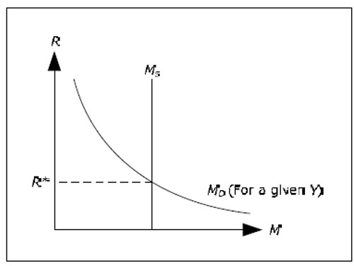
Fig. 12.1
In the diagram above, R* is the interest rate in which the demand for money is exactly equal to the supply of money (again for a given Y ). The IS-LM model, R will always tend to R* until they are equal and we have an equilibrium in the money market.
The justification for why R will tend to R* is not entirely straightforward:
- Say that R < R*.
- In this case, MD > MS , that is, people want to hold more money than what is available.
People increase the amount of money they hold by selling bonds so there is an excess supply of bonds.
- This excess supply of bonds will drive down the price of bonds.
- When the price of bonds falls, interest rates increase. We discussed this negative relationship between the price of bonds and the interest rate in section: The yield curve.
- The interest rate will increase until R = R*. Only then will the demand for money have decreased enough such there is no longer an excess demand for money. Then there is no excess supply of bonds either. The money market is in equilibrium.
- The case of R > R* can be analyzed in the same way.
The money market diagram can be used to determine the equilibrium rate of interest if we know GDP.
IS-LM diagram
IS Curve (Investment-Savings)
The IS curve shows all combinations of R and Y where the goods market is in equilibrium. The IS-curve slopes downwards.
The goods market is in equilibrium when YD(Y, R) = Y. Note that when R is given, the IS-LM simplifies to the cross model:
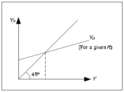
Fig. 12.2
If we know R, we can determine the equilibrium value of Y using the cross model. Also, if we know Y we can determine R from the money market. None of the methods, however, will gives us both R and Y simultaneously.
Consider the following question: What must happen to Y when we change R if we want the goodsmarket to remain in equilibrium? To answer this question, consider two different interest rates, R1 = 5% and R2 = 10%. Since YD depends negatively on R, YD(Y, R1) will be larger than YD(Y, R2). With a higher R, we must have a lower Y for the goods market to be in equilibrium.
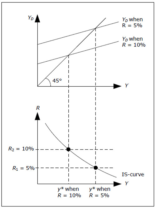
Fig. 12.3
We can illustrate this argument with the above diagram.
- Start by identifying R1 and R1 in the lower graph.
- Draw aggregate demand for both interest rates – the one corresponding to the lower interest rate will be higher than the other.
- Identify the resulting GDP in the upper diagram for both interest rates – the highest level of GDP corresponds to the lower interest rate.
- Extend these levels of GDP to the lower graph. This will give you two points in the lower graph.
- Continue with other interest rates if you like. The result will be a curve in the lower graph that we call the IS-curve.
The IS curve will identify all combinations of Y and R where YD(Y, R) = Y, that is, where the goods market is in equilibrium. The economy must be on this curve if the commodity market is to be in equilibrium. However, an analysis of the goods market alone will not help us identify at which point all markets are in equilibrium. Note that the cross model is represented by a single point on the IScurve – the point corresponding to the exogenously given interest rate. This is why we can determine Y in cross model only from the commodity market.
The IS Curve: Goods Market Equilibrium
The IS curve represents combinations of interest rates and output (GDP) where the goods market is in equilibrium. It is derived from the Keynesian national income identity:
Y = C + I + G +(X - M)
Where:
- Y is national income/output,
- C is consumption,
- I is investment,
- G is government spending,
- X - M is net exports (exports minus imports).
The IS curve is downward sloping because an increase in interest rates discourages investment, leading to a decrease in aggregate demand and national income. Conversely, a lower interest rate stimulates investment, increasing output.
The LM curve
The LM curve shows all combinations of R and Y, where the money market is in equilibrium. The LM-curve slopes upwards.
The money market is in equilibrium when Md(Y, R) = Ms. In section 12.3.6 we demonstrated how the money market diagram will determine R when we know Y. In this case, the question to consider is the following: What must happen to R when we change the Y if we want the money market to remain in equilibrium?
To answer this question, we try two different values for GDP Y1 = 100 and Y1 = 200. Since the MD depends positively onY, MD(Y1, R) will be smaller than the MD(Y2, R). R must therefore be larger when Y increases for the money market to be in equilibrium.
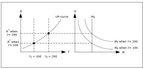
Fig. 12.4 Derivation of the LM-curve.
The diagram above illustrates this point.
- Start by selecting Y1 and Y2 in the left graph (Y2 < Y2).
- Draw the money demand for each of the different levels of GDP in the diagram to the right – the one corresponding to the lower value of GDP must be the smallest.
- Identify the resulting interest rate in the diagram to the right for both levels of GDP – the larger of the interest rates corresponds to the larger value of GDP.
- Extend these interest rates to diagram on the left. This will give you two points where the money market is in equilibrium.
- Continue with the other levels of GDP. The result will be a curve in the left diagram that we call the LM-curve.
The LM curve will show you all combinations of Y and R where Md(Y, R) = Ms, that is, where the money market is in equilibrium. Again, the economy must be on the LM curve if the money market is to be in equilibrium and the money market alone cannot determine which point will lead to equilibrium in all markets.
The LM Curve: Money Market Equilibrium
The LM curve represents equilibrium in the money market, where money demand equals money supply. It is based on the Keynesian theory of liquidity preference, which states that people hold money for three reasons:
- Transactions Motive: To conduct daily transactions.
- Precautionary Motive: To guard against unexpected expenses.
- Speculative Motive: To take advantage of changes in interest rates.
The equilibrium condition in the money market is given by:
Ms = Md
Where:
- Ms is the money supply,
- Md is the money demand, which depends on income and interest rates.
The LM curve is upward sloping because higher income levels lead to higher money demand, pushing up interest rates to maintain equilibrium.
Simultaneous determination of Y and R in the IS-LM model
By combining the IS curve and the LM curve, we can graphically illustrate what interest rate and what level of GDP that will satisfy both equations: YD(Y, R) = Y and MD(Y, R) = MS. For all points on the IScurve,we have equilibrium in the goods market and for all points on the LM-curve, we have equilibrium in the money market. There is only one point where both markets are in equilibrium, Y* and R*.
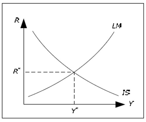
Fig. 12.5:IS-LM model.
According to IS-LM model, the economy will move to Y* and R*. The argument is as follows.
- Imagine that R > R*. It is the not possible to be on both the IS and the LM-curve.
- Suppose that we are on the IS-curve, but to the left of the LM curve. The interest rate is higher than the equilibrium interest rate and R will fall as discussed in 12.3.6.
- Suppose that we are on the LM-curve, but to the right of the IS-curve. Y is then higher than the equilibrium value and Y will fall as discussed in 11.3.2. We will then move away from the LM-curve and the interest rates will fall.
- If we are neither on the IS- nor on the LM-curve, then Y will fall as long as we are to the right of the IS-curve and R will fall as long as we are to the left of the LM-curve.
The Labor Market
The labor market in the IS-LM model is the same as in the cross model. Therefore, the IS-LM model is only applicable if the profit-maximizing quantity of L would lead to an aggregate supply that was larger than the aggregate demand and aggregate demand will therefore determine L. Once R and Y is determined, all the endogenous variables are determined. The diagram below shows the determination of Y, R and L in the IS-LM model.
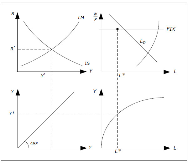
Fig. 12.6: Determination of Y, R and L of the IS-LM model.
We start at top to the left and extend Y* down, through the “mirror” at the bottom left, on to the production function at the bottom right and then up to the diagram representing the labor market. The IS-LM is simply an extension of the cross model in the sense that the interest rate becomes an endogenous variable and we will be able to analyze how the interest rate is affected by changes in the economy.
We could have developed the IS-LM model directly, skipping the cross model as the cross model adds nothing in relation to the IS-LM model. The reason that most books (including this one) start with cross model is entirely pedagogical. The cross model is much simpler since GDP can be determined from the goods market only as the solution to one equation one equation Yd(Y) = Y. Most students would probably find the Investment Saving, Liquidity preference Money supply IS-LM model even more complicated had they not previously encountered the cross model.
IS-LM Equilibrium
The intersection of the IS and LM curves determines the short-run equilibrium level of interest rates and output. This equilibrium represents a situation where both the goods and money markets are in balance simultaneously.
Fiscal Policy in the IS-LM Model
Fiscal policy, which involves changes in government spending and taxation, affects the IS curve.
- Expansionary Fiscal Policy (Increased G or reduced T): Shifts the IS curve to the right, increasing output and interest rates.
- Contractionary Fiscal Policy (Reduced G or increased T): Shifts the IS curve to the left, reducing output and interest rates.
The effectiveness of fiscal policy depends on the slope of the LM curve. If the LM curve is steep (money demand is highly responsive to income changes), fiscal policy has a weaker effect on output and a stronger effect on interest rates.
Monetary Policy in the IS-LM Model
Monetary policy, which involves changes in the money supply, affects the LM curve.
- Expansionary Monetary Policy (Increased money supply): Shifts the LM curve to the right, reducing interest rates and increasing output.
- Contractionary Monetary Policy (Decreased money supply): Shifts the LM curve to the left, increasing interest rates and reducing output.
The effectiveness of monetary policy depends on the slope of the IS curve. If the IS curve is steep (investment is not highly sensitive to interest rates), monetary policy has a weaker effect on output and a stronger effect on interest rates.
Limitations of the IS-LM Model
While the IS-LM model is a useful tool for analyzing macroeconomic policies, it has several limitations:
Short-run Focus: The model does not incorporate long-term economic growth factors such as technological progress and capital accumulation.
Fixed Price Level: The model assumes fixed prices, making it less applicable in an inflationary environment.
Closed Economy Assumption: The traditional IS-LM model does not account for international trade and capital flows.
Simplified Monetary Sector: The model does not capture complexities in the financial system, such as credit markets and banking dynamics.
Conclusion
Despite its limitations, the IS-LM model remains a foundational framework in macroeconomics. It provides valuable insights into how fiscal and monetary policies influence interest rates and output in the short run. While modern macroeconomic models have evolved, incorporating dynamic and open-economy perspectives, the IS-LM model continues to serve as a useful starting point for understanding macroeconomic policy interactions.
By understanding the IS-LM framework, policymakers and economists can better analyze economic fluctuations and design policies to stabilize the economy. Whether for academic purposes or practical policymaking, mastering the IS-LM model is essential for anyone interested in macroeconomic analysis.