Exchange rate determination and the Mundell-Fleming model
- Details
- Category: Macroeconomics
- Hits: 20,472
The open economy
So far, our model for exchange rate determination has been very simple. We have assumed that domestic interest rates are unaffected by foreign interest rates. We begin this chapter by looking more carefully at this assumption (the classical model of exchange rate determination). Then, a more realistic model of exchange rate determination is considered.
Finally, we will discuss the Mundell- Fleming model (MF-model).
The Mundell-Fleming model is a model for an open economy. Such models must consider the determination of the exchange rate and how the exchange rate affects imports and exports. They also typically assume that capital may move freely and that investments will flow to countries where the return is maximized.
The Mundell-Fleming model is probably the simplest among the many macroeconomic models of the open economy. The Mundell-Fleming model is basically an extension of the neoclassical synthesis with a model for the exchange rate that allows for free capital flows.
The rest of the world as one country
Most of the open economy models treat the rest of the world as one country. Focus on these models is on aggregate exports and imports and we are less interested in which particular countries we trade with. The same argument applies to capital flows. In these models, the rest of the world will have a single currency that we call the foreign currency. Therefore, there are only two currencies (the foreign and the domestic) and a single exchange rate.
Exchange rate systems
For an open economy, the particular exchange rate system in use becomes important. In exchange rate we discussed some possible systems. In simple models, only two systems are considered: a floating or a fixed exchange rate.
- With a floating exchange rate, the exchange rate is determined as any price, that is, by supply and demand. The central bank never intervenes in the market.
- With a fixed exchange rate, the exchange is completely fixed. In reality, most countries with a fixed rate allow the exchange rate to vary within certain limits. These variations are disregarded and the central bank will always intervene to keep the exchange rate at its fixed value.
Also, remember the following notation:
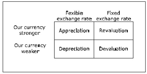
Fig. 16.1: Changes in exchange rates.
The classical model of exchange rate determination
The classical model of exchange rate determination is the one we have used so far. This section will consider the foundations of this model
The law of one price
The classical model for exchange rate determination is based on the law of one price. This law claims that there can be only one price for a given product at any given time. Gold, for example, must cost more or less the same wherever you buy it.
If gold was traded for USD 30,000 per kilo in New York and for USD 40,000 per kilo in Chicago, you would be able to make a lot of money by buying gold in New York and selling it in Chicago. There would be opportunities for arbitrage – opportunities to make money with no risk. Gold would be transported from New York to Chicago until the price difference was eliminated.
The law of one price need not apply exactly due to the following reasons:
- Transportation costs: If the price difference is less than the cost of transport, the difference may remain.
- Ease of access. A soda in a convenience store is often more expensive than in a supermarket. You pay slightly more for the convenience of the ease of access.
- Government intervention. The government may, for example, by subsidizing electricity for firms, create a market with two different prices for the same good.
For non-transportable goods and services, the price difference may be much larger. Even if the price of a haircut is much higher in Chicago than in Boise, Idaho, there are no strong arbitrage possibilities that will remove the price difference.
Purchasing Power Parity (PPP)
If we apply the law of one price to goods in different countries, we can derive the purchasing power parity (PPP). If gold is trade in the U.S. at USD 30,000 per kilo and 1 euro costs USD 1.40, you can be pretty sure that gold will trade for around 30,000/1.4 ≈ 21,400 euros per kilo. If that was not the case, there would again be arbitrage opportunities (unless there are restrictions on transporting gold across borders). If PF is the price of a good in the foreign country, P is the price of the same good in our country and E is the exchange rate (domestic/foreign) then PPP claims that P = PF*E
The Big Mac Index
Based on PPP, the Economist regularly publishes the "Big Mac Index". PF is then the price of a Big Mac in the U.S. . In February of 2009, PF was on average 3.54 USD and exchange rate E = 1.28 USD / euro. According to PPP, a Big Mac should cost 2.77 euros in the euro area. In reality, it costs on average 3.42 euros. We would need an exchange rate of 3.54 / 3.42 = 1.04 USD / euro for the PPP to be entirely correct for the Big Mac.
According to Big Mac index, the euro is overvalued by about 24% in relation to the USD. The most expensive Big Mac, however, is found in Norway. Here a Big Mac costs USD 5.79 at the current exchange rate making the Norwegian krona overvalued by 63%.
Exchange rate determination
In PPP, PF and P denote the domestic and foreign price of a particular good. If we instead let PF and P denote price levels, we can derive the classical model of exchange rate determination simply by dividing both sides in PPP by exchange rate E:
E = P/PF
If the UK is our home country and a basket of goods costs 12.0 million UK pounds (GBP) while the exact same basket costs 14.1 million euro in France, the exchange rate, according to the classical model, ought to be 0.851 GBP/EUR or 1.175 EUR/GBP.
The exchange rate that we just calculated is often called the purchasing power adjusted exchange rate. If this was the actual exchange rate, the price levels (in the same currency) in the two countries would be the same. When we compared GDP per capita for various countries in section 3.6, it was the purchasing power adjusted exchange rate that we used to transform GDP into the same currency.
For countries where the GDP per capita is very different, the actual exchange rate is often very far from the purchasing power adjusted exchange rate. The price level in countries with a high GDP per capita is generally higher than the price level in countries with a low GDP per capita (in the same currency). It is often for services and non-transportable goods where prices deviate the most.
Inflation
If the price level in the home country and the foreign price level do not change, then, according to the classical model of exchange rate determination, exchange rate E will be constant. The same is true if P and PF increase at the same rate, that is, if the home country has the same inflation as the rest of the world: π = πF, where πF is the rate of inflation abroad.
If, however, π > πF (P increases faster than PF), then exchange rate E will increase (our currency will depreciate). For example, if π = 8% while πF = 5%, P increases by 8% while the PF increases by 5% over the same period. P/PF will then be 1.08 / 1.05 ≈ 1.03 times larger than the old value, that is, exchange rate E will increase by about 3%. Our currency will have depreciated by 3% during this period.
If πE is the rate of increase in the exchange rate (the rate that our exchange rate depreciates), the classical model predicts:
πE ≈ π − π F
The rate of depreciation is (approximately) equal to the differences in inflation between the countries.
In the exercise book, we show that the exact relationship is 1 + πE = (1 + π)/(1 + πF) and the difference between these two results is small if inflation ratess are not too high.
Differences in inflation under fixed exchange rates
Suppose that we have a fixed exchange rate with a foreign country (rest of the world) but that we have different rates of inflation. Say that π F = 0 while π = 10% – our prices increase 10% annually (in our currency) while foreign prices are stable (in their currency).
If the exchange rate is fixed, domestically produced goods will also increase by 10% per year in the foreign country. As they have stable prices, the demand for our goods will continually decline.
Also, import prices in our country will remain unchanged but since the price of domestic products increases by 10% per year, imported goods will continuously become cheaper and cheaper relative to domestically produced goods and imports will increase. Such a situation is unsustainable in the long run – we will eventually be forced to devaluate our currency. To keep a fixed exchange rate between two countries, it is necessary that these countries have the same inflation.
Differences in inflation under flexible exchange rates
With flexible exchange rates, no such restriction exists – countries may have different rates of inflation and no problem with trade need to occur. To see why, imagine again that πF = 0 while π = 10% (per year) but that πE = 10% as the classical model predicts. Our country has inflation of 10% and our currency loses 10% of its value each year.
Say that Germany is our home country and that a domestically produced machine costs 10 EUR (in millions or whatever). At the same time, foreign-produced computer costs 4 USD. The exchange rate at this time is 0.711 EUR/USD. The machine will then cost 14.05 USD abroad while the computer will cost 2.85 EUR in Germany.
One year later, the price of the machine has increased to 11 EUR in Germany while the price of the computer has not changed. Also, the euro has lost 10% ( E has increased by 10%) and the new rate is 0.783 EUR/USD. The price of the German machine abroad is still 14.05 USD (11 / 0.783) and exports will not be affected. Further, the price of the foreign-produced computer has increased to 3.13 EUR in Germany, an increase of exactly 10%. Since all other prices increase by 10% in Germany, imports will not change either.
We note that under flexible exchange rates, as long as the exchange rate depreciates at a rate equal to the difference in the rates of inflation, we may assume that exports and imports are unaffected by changes in the price levels and the exchange rate. This is exactly the assumption we have made so far.
The exchange rate
We now include capital flows between countries. We denote the foreign currency by the symbol $ while € denotes the domestic currency. Remember that the exchange rate E is the units of € we need to buy one unit of $. For example, E = 0.8 €/$ means that $1 costs 0.8€. That in turn means that €1 costs $1.25. Note that if E is the exchange rate in €/$ then 1/E is the exchange rate in $/€.
In principle, there are two reasons for selling or buying currency:
- Trade and tourism
- Foreign investment
Trade and tourism
Domestic firms that import goods from abroad must pay for the goods using $. Since they are paid in €, they will continuously need to sell € and buy $. Domestic import firms create a demand for $. People in our country that visits foreign countries will also contribute to this demand.
Foreign firms that import goods from our country must pay in €. They thereby create a demand for €. Whenever there is a demand for €, there will be a simultaneous supply of $. Foreign importers create a supply of $ (foreign tourists also contribute to this supply). Note that even though foreign importers pay in $, the end result will be the same. If domestic exporters receive payments in $, they will contribute to the supply of $ as they have expenses in €.
Imports create a demand for $
Exports create a supply of $
Capital flows
Another factor that contributes to the demand and supply of $ are capital flows. If someone in our country wants to invest abroad, she must first buy $ thereby adding to the demand for $. In the same way, foreigners who want to invest in our country must first buy € and they will contribute to the supply of $.
Domestic investments abroad add to the demand for $.
Foreign investing in our country adds to the supply of $.
Trade and exchange rate
We begin by analyzing how exchange rate E affects exports and imports (X and Im). Imagine first that E = 0.8 €/$. A product that costs $100 abroad will cost €80 in our country (ignoring transportation costs and other factors affecting the validity of PPP). A domestic product costing €100 will cost $125 abroad. Say that exchange rate E increases to 0.9 €/$ (everything else the same). € has depreciated or has been devalued and is now weaker against $. The $100 good now costs €90 in our country.
Foreign-produced goods have become more expensive in our country and imports will decrease. The €100 goodwill now costs $111 abroad. Domestically produced goods have become cheaper abroad and exports will increase. Depreciation or devaluation (E up = weaker currency): X increases, Im decreases Appreciation or revaluation (E down = stronger currency): X decreases, Im increases
This is true if everything else is the same, an important qualification as we will soon see.
Investment and the exchange rate
When you invest money abroad, the future exchange rate at the time when you want to transfer your funds back to your country is important. Say for example that you invest €1 million in a foreign
country at a 10% interest rate. When you make the investment, E = 0.8 €/$ which means that you invest $1.25 million. After one year, this amount has increased to $1.375 million. If the exchange rate is the same one year later, this amount is equal to €1.1 million and your return is 10%. If, however, our currency has strengthened and E = 0.4 €/$, the amount $1.375 million will only give you €0.55million, and you have lost 45% of your investment! On the other hand, if € has weakened and E = 1.6 €/$ a year later, you will now receive €2.2 million, a nice return of 120%.
From this example, we can figure out how the exchange rate E affects capital flows. Suppose that the expected exchange rate one year from now is 0.8 €/$. If E = 0.8 €/$ today, we expect to neither gain nor loose fromchanges in the exchange rate from investments within the next year.
If exchange rate E increases to 0.9 €/$ today while the expected exchange rate remains at 0.8 €/$, those who want to invest abroad for one year will expect to make a currency loss (they buy the $ for 0.9€ and can expect to sell it a year later for 0.8€). At the same time, foreigners who invest in our country can expect to profit from the expected change in the exchange rate. When the current E increases (with a fixed future E), investing abroad will be less attractive while investments in our country will be more attractive.
E up = weaker currency: fewer investments abroad, more investments in our country
E down = stronger currency: more investments abroad, less in our country
Again, this assumes that everything else is the same (in particular, the expected future exchange rate).
Supply and demand for the foreign currency
We denote the supply and demand for the foreign currency by S$ and D$. S$ will depend positively on the E and D$ will depend negatively on E. The reason is as follows:
-
When exchange rate E increases (weaker currency) exports will increase, imports will fall, investments abroad will fall and investments in our country will increase.
-
Increasing export will increase the supply of $ (S$ up)
-
Decreasing imports will decrease the demand for $ (D$ down)
-
More investments in our country will increase the supply of $ (S$ up)
-
Fewer investments abroad will decrease the demand for $ (D$ down)
With a completely floating exchange rate, the exchange rate is determined in the same way as any other price:
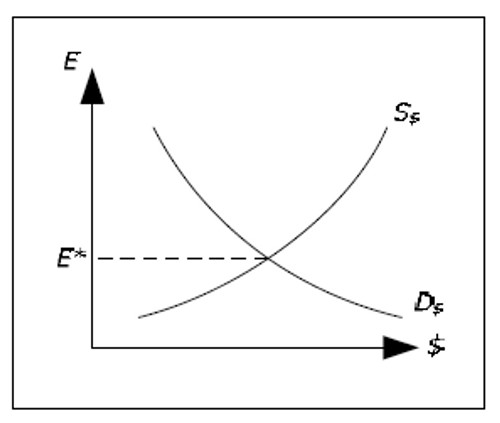
Fig. 16.2 Exchange rate determination.
E* is the equilibrium exchange rate, the exchange rate where S$ is equal to D$. If the currency market is a free market, E will be equal to E*. With a fixed exchange rate, the central bank must be prepared to buy and sell currency at the predetermined exchange rate.
Factors affecting the exchange rate
A large number of factors may affect E*. Some examples:
- Higher growth in domestic productivity. This would make domestic products cheaper and the demand for € would increase. This would increase the supply of $ and E* would fall (stronger currency).
- Higher domestic inflation. This would make domestic products more expensive and the domestic currency would depreciate.
- Higher domestic interest rates. This would increase the demand for € and the currency would strengthen.
Mundell-Fleming model
One of the main assumptions in the Mundell-Fleming model is the assumption of interest rate parity. We begin by explaining this assumption.
Interest rates within in the same currency area
A currency area is a geographic area where the same currency is used. The United Kingdom is one example of a currency area and all the countries using the euro is another (France, for example, is not a currency area, as they use the euro).
Within a currency area, at a certain point in time, there can be no significant differences in the interest rate geographically. With large differences, there would be arbitrage possibilities (the argument is similar to that of the law of one price). If it was possible to borrow/lend at interest rates 6% / 5% in Paris and at the interest rates 4% / 3% in Athens, you could become very wealthy.
Interest rates between currency areas
Between currency areas, it is not as simple. Even if you can borrow at 4% in one area and lend at 5% in another, you cannot be sure that you will make a profit. The reason, of course, is that the exchange rate may change and what you gain from the interest rate differential, you lose from changes in the exchange rate.
However, if you somehow knew that the exchange rate would be the same in the future, then the interest rates would have to be the same. But even with fixed exchange rates, you cannot know this for sure as exchange rates may be devalued or revalued.
Expected depreciation
To figure out the relationship between the domestic interest rate R and the foreign interest rate RU we introduce the concept expected depreciation: πE e. The expected depreciation indicates how much investors expect the domestic currency to lose against the foreign currency within a given period. For example, if exchange rate E = 0.8 €/$ today and it is expected that E = 1 €/$ in one year, the expected depreciation is equal to 25%, πEe = 0.25. If you expect an appreciation of say 10%, we write πEe = –0.1.
Interest rate parity
An important assumption in the Mundell-Fleming model is the assumption of interest rate parity:
R ≈ RU + πEe
The domestic interest rate should be approximately equal to the foreign rate plus the expected depreciation. If the foreign one-year interest rate is 3% and you expect our currency to lose 2% to the foreign currency, then, according to the interest rate parity, the domestic one-year interest rate should be approximately 5%. The exact result is 1 + R = (1 + RU)(1 + πEe) or R = 5.06%.
Interest rate parity can be justified using arbitrage arguments. If interest rate parity holds, the expected return abroad will be the same as the domestic return and there will be no major flows of capital ineither direction.
Say again that R = 5%, RU = 3%, πEe = 2% and E = 0.8 €/$ initially. If you invest 1000 in the euro area, you have 1050 after 1 year. If you invest them abroad, you invest $1250. At 3%, you have $1287.5 a year later. If the actual depreciation is equal to the expected, E = 0.816 one year later. $1287.5 at the rate 0.816 €/$ is approximately equal to 1050.
Note that the actual rate of return may differ between countries if the actual appreciation differs from the expected depreciation. However, as long as expected returns are the same, there will be no major movements affecting the current exchange rate.
Modeling expected depreciation
Fully-extending the neoclassical synthesis to an open economy is not simple. The main reason for this is that we need a model for how expectations on the exchange rate are formed. A simple solution to this problem is to assume that expectations are exogenous. In more advanced models, expectations are endogenous. Fortunately, a simple model with exogenous expectations leads to results that are similar to more complex models with endogenous expectations.
We assume that πEe = 0 if the exchange rate is fixed. In practice, this means that we do not expect any devaluations or revaluations. With πEe = 0, R = RF.
We assume that πEe = π − πF in the long run if the exchange rate is flexible. If domestic inflation is 4% above the rest of the world, we expect a 4% depreciation of the exchange rate. In the short run, πEe is assumed to be fixed (and equal to the inflation differentials in the last period).
If our country is small in relation to the rest of the world (the foreign country), it is reasonable to assume that RF is determined as if the foreign "country" was a closed economy while our interest rate R is affected by RF. With fixed exchange rates, our interest rate is simply equal to the world interest rate. With a flexible exchange rate, our interest rate is equal to the world interest rate plus or minus a given constant (πEe).
The IS-LM model under fixed exchange rates
With fixed exchange rates, R is given. We can illustrate this by drawing a new curve in the IS-LM diagram called the FE-curve (FE for Foreign Exchange).
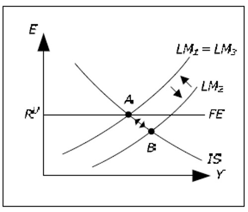
Fig. 16.3: IS-LM-FE.
We have drawn the diagram such that the IS curve intersects the LM curve at exactly the "correct" interest rate R = RU. This is no coincidence – we will describe why the IS curve must intersect the LM curve at exactly this interest rate. Let us begin by analyzing what will happen when MS increases when we are initially in equilibrium (with say πM = π = 0).
- The LM curve shifts outwards from LM1 to LM2. We move from A to B.
- Y falls and R falls. Now R < RF and the demand for foreign currency increase.
- Our currency will depreciate and the central bank must intervene. They will sell foreign currency and buy the domestic currency which will reduce foreign exchange reserves.
- When they buy domestic currency, Ms will fall. LM2 shifts back towards LM1 and the process will continue until R again is equal to RF, LM2 is back to LM1 and we are back at point A.
Monetary policy has no effect when the exchange rate is fixed according to the Mundell-Fleming model. However, as we shall see in the exercise book, fiscal policy will work. Fiscal policy will actually work better in the open economy than in the closed economy. In reality, results are not so black and white. Instead, you should conclude that monetary policy is less effective with a fixed exchange rate – not that it is completely ineffective.
The IS-LM model with flexible exchange rates
With flexible exchange rates, we must also consider the expected depreciation, R = RF + πEe. Since πEe is assumed to be exogenous, the FE curve is still horizontal.
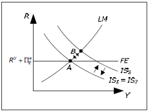
Fig. 16.4: IS-LM-FE.
In this case, we analyze what happens when G increases from an initial equilibrium (again, πM = π = 0).
- The IS curve shifts outwards from IS1 to IS2. We move from A to B.
- Y increases and R increases. Now R > RF + πE e and the supply of foreign currency increases (foreigners will want to buy our currency and invest in our country).
- Since we have a flexible exchange rate, the central bank will not intervene and the domestic currency will appreciate it.
- When the domestic currency appreciates, exports will fall while imports will increase. This will shift the IS2 curve back towards IS1. The exchange rate will continue to appreciate as long as R > RF + πEe and the trade balance will continue to deteriorate until R again is equal to RF +πEe and IS2 is back to IS1.
Fiscal policy has no effect under flexible exchange rates according to the Mundell-Fleming model. Any attempt to stimulate the domestic economy will only succeed in stimulating the foreign economy. However, as we shall see in the exercise book, monetary policy will work (and in this case better than in the closed economy)