Oligopoly

An oligopoly is a market in which there are only a few sellers. Most of the models in the literature only cover cases in which there are two sellers. Such markets are also called duopolies. As you will see, the analysis of oligopolies is quite complicated. Furthermore, there are several different models that yield different results. This can be quite confusing. Take some time to see what the differences are in the assumptions and why they give different results. Which model to use, depends on what the situation is in a particular case. Different structures can have dramatically different effects on the market.

Kinked Demand Curve

Assume there are only a few firms in a market and that they all produce exactly the same good. Furthermore, assume that there is already a price has already been set. (For now, we will ignore the question from where this price has come.) If we were one of the firms, how would we reason regarding our own price setting?

What would happen if we would raise the price? Most of the customers would then buy from our competitors instead, to get good at a lower price. The competitors would probably not lower their prices, as they would gain a larger market share instead. Consequently, we would sell much fewer goods. Conversely, what would happen if we lowered our price? If the competitors did not also lower their prices, we would gain a large part of their market shares. Since that would mean that they would reduce their profits, they would probably lower their prices as well.

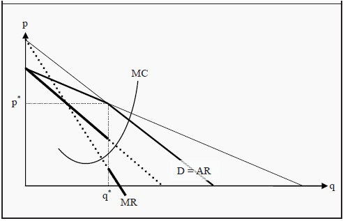
Figure 14.1: Kinked Demand Curve

The slope of the demand curve that our firm faces is therefore different depending on whether we increase or decrease our price. This results in a so-called kinked demand curve, where the bend occurs at the existing price, p*, and the corresponding quantity, q* (see Figure 14.1).

The bend in the demand curve makes the construction of the MR curve more complicated. To find the MR curve, we extend the two parts of the demand curve, D, until they reach the two axes. (The extensions are the thin lines in the figure.) As the (real and imagined) demand curves are downward sloping, their corresponding MR curves will also be downward sloping, intercept the Y-axis at the same points, but have a slope which is twice as large. (Compare to the reasoning regarding the MR curve of a monopoly, Section: Demand and Marginal Revenue) Since D now has two parts, we do this for each part separately.

Since the demand curve is bent at the quantity q*, the MR curve will also change at that quantity. To the left of q*, we use the MR curve that is derived from that part of the demand curve that is valid to the left of that quantity. To the right of q*, we instead use that MR curve that is derived from the part of the demand curve that is valid to the right of it. This causes the final MR curve to making a jump at q*. In Figure 14.1, the final MR curve is indicated with thick full lines. The parts that are not used, since they correspond to the extensions of the demand curve, are indicated with thick dotted lines.

Just as before, a criterion for profit maximization is that the firm sets the quantity where MR = MC. In the models we have used this far, that criterion singled out exactly one point. However, since the MR curve now makes a jump at the quantity q*, the MC curve can intersect the MR curve in that interval. At the prevailing price, it must do so by construction. This means that if the marginal cost, MC, only changes a little bit, for instance, because a small tax is introduced on each unit sold, the firm might not change its produced quantity, and consequently not the price. As long as the MC curve still intersects the MR curve at the jump, the firm will produce the same quantity, q*. However, the increase in MC will lead to a reduction in profit for the firm.

This is one way that the real-world phenomenon of sticky prices can be explained.

According to the previous market-models (perfect competition and monopoly), prices should change immediately if quantities change. However, often we see that prices change more seldom; they seem to be stuck at a certain level for a while. If prices and quantities are set according to the kinked demand curve-model, however, this is exactly what we should expect.

How does the Price in the Kinked Demand Curve Arise?

In the analysis in the last section, we ignored the question of how the price had risen. One idea is that the sellers can have agreed on the price. If sellers can cooperate on the price setting, they will optimally agree to set a price that corresponds to the quantity a monopoly would have chosen, since the monopoly profit is the largest one can possible make in a market. Then they could split the monopoly profit between themselves. However, that would amount to setting up a cartel, and that is against the law. Many people argue, however, that firms can have tacit agreements. There is no real cartel, but there is a sort of silent agreement that each seller should set a high price. A frequently used example is the way gasoline distributors set their prices. Often, one firm announces that it will increase its price. Then the other firms follow immediately. Note, however, that this type of behavior can also be against the law.

Cournot Duopoly

The Cournot model is a model of duopolies and is developed in line with the game-theoretical approach we presented in last chapter. The Cournot model assumes that:

• We have two firms.
• They set quantities (and the price is then set by the market, given the quantity).
• They choose simultaneously, without knowing which quantity the other chooses.

How would these two firms reason? Both of them want to maximize their own profit. However, each firm’s profit partly depends on the quantity set by the other firm, as total quantity determines the market price.

If a firm knows the quantity the other firm has chosen, then it is able to decide exactly which quantity that would maximize their own profit. There is an optimal response to each choice of the other firm. Let us use that observation, and determine that best response for each choice of quantity the other firm can possibly make. If we do that, we get a so-called reaction function. In Figure 14.2, r1 is firm 1's reaction function and r2 is firm 2's.

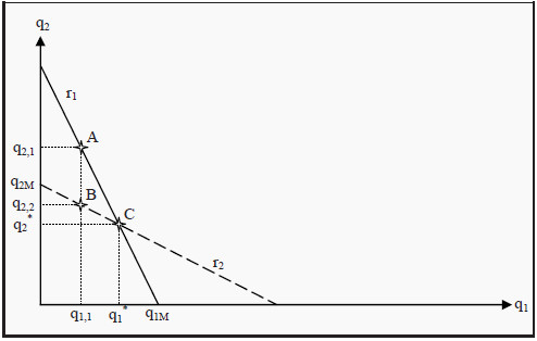
Figure 14.2: The Cournot Model

To give an example of how to interpret the reaction function, suppose that firm 2 chooses to produce the quantity q2,1. Which is firm 1’s optimal response? Indicate q2,1 on the Y-axis, go to line r1 (point A) and read off the corresponding value on the X-axis: q1,1 is firm 1's optimal response. Note however that if firm 1 chooses the quantity q1,1, then the quantity q2,1 is not optimal for firm 2. Instead, the quantity q2,2, at point B, is optimal for firm 2. However, then q1,1 is not optimal for firm 1… and so on.

It is possible to show that the only point where both firms simultaneously respond optimally to the other’s choice is point C, where the two reaction curves intersect each other. As no agent can achieve a better outcome by unilaterally changing her strategy, we have a Nash equilibrium (see Section: Nash Equilibrium). The conclusion of the Cournot model is then that, both firms will choose the Nash equilibrium quantities, q1* and q2*. Note that, if you continue to use the method of finding successive optimal responses as we did above, you will tend to get closer and closer to the Nash equilibrium in each round.

One should also note another thing in Figure 14.2. If firm 2 would produce nothing at all, firm 1 would be a monopolist in the market. The optimal quantity would then be the monopoly quantity. Similarly for firm 2. The reaction function of each firm must consequently hit the firm’s own axis at the monopoly quantity. In the figure, these points are labeled q1M and q2M.

Stackelberg Duopoly

In the Cournot model, both firms made their decisions simultaneously and without knowing the other’s decision. In the Stackelberg model, they decide one after the other. We call the one that chooses first, the Leader and the other one the Follower.

• We have two firms.
• They set quantities (and the price is set by the market).
• The leader first decides on her quantity, and then Follower decides on hers.

We will use the same reaction function as in the Cournot model, but the analysis will now be different since they do not choose simultaneously. A leader, who sets her quantity first, has an advantage. She knows that Follower will later set her quantity according to her reaction function. Therefore, the Leader sets her quantity to maximize her own profit, given Follower’s optimal response.

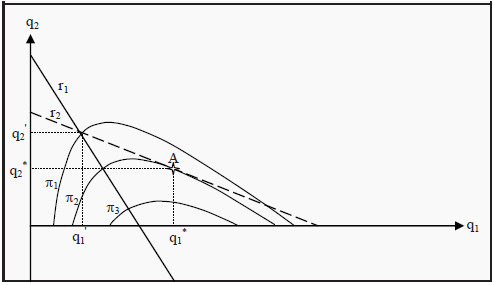
Figure 14.3: The Stackelberg Model

One way to illustrate this game is presented in Figure 14.3. We have drawn the reaction functions, r1 and r2, but we have also added a few curves indicating Leader's profit, π1, π2, and π3; so-called isoprofit curves. Such curves show different combinations of q1 and q2 that give the Leader the same profit. For instance, all combinations along π1 give Leader a profit of π1, etc. Note that Leader's profit increases inwards, the closer to the monopoly quantity (the point where r1 intersects the X-axis) we get.

The profit at π2 is consequently higher than at π1, and even higher at π3. Leader knows that Follower will choose her quantity along the reaction function r2. Leader therefore finds an isoprofit curve that touches r2 and that is as close to the monopoly quantity as possible. In the figure, the isoprofit curve π2 touches r2 in point A. Leader then chooses the quantity that corresponds to point A, i.e. q1*. As a response, Follower later chooses the quantity q2*.

Note that every other choice of quantity for Leader, higher or lower, must result in a lower profit for her. If she, for instance, would choose the quantity q1 ' instead, Follower's reaction would be to choose q2' and Leader's profit would be π1, which is less than π2.

Bertrand Duopoly

In the two preceding models, we have assumed that the firms set quantities. What happens if, instead, they set prices? The Bertrand model assumes that:

• We have two firms.
• They set prices (and quantities are set by the market).
• They set prices simultaneously, without knowing which price the other one sets.

The previous models produced results that were very favorable for the firms but less so for the consumers. The Bertrand model, however, puts the two firms in a Prisoner’s Dilemma-type of the situation (see Section: The Prisoner’s Dilemma), and forces them to set p = MC, i.e. they set the same price as firms would do in a perfectly competitive market. This is, of course, unfavorable for the firms, but an improvement for consumers and society.

To see that the firms will set p = MC, suppose that we know that the other firm has set a high price. Which is then the best price we can set? Remember that we have homogenous (meaning identical) goods, so the consumers will not care from whom they buy it. Furthermore, they have perfect information about all prices. If we choose a price that is just below our competitor’s, all customers will buy from us. This is a good situation for us, but far from optimal for the other firm. If the reason in the same way, they will want to set a price just below ours. Then we would lose all customers… and so forth.

No price above MC can consequently be an equilibrium. Regardless of which price the firm has set, the other will always want to undercut it and set a price just below its competitor. The only price that can be an equilibrium is then p = MC. At that price, none of the firms can lower their price since they would then make a loss. None of them would be able to make a profit by increasing the price either, since they would then lose all customers.

The surprising result is then that, since p = MC, we get the same outcome as in a perfectly competitive market, even though there are only two firms. If society is able to construct an oligopoly such that it becomes a Bertrand duopoly, there will be no loss of efficiency.

One way for the firms in a Bertrand market to increase profits anyway, is to try to differentiate their products. The customers will then not be indifferent between from whom they buy and the firms become two monopolists, however with goods that are very close substitutes. We will look at this type of situations in Monopolistic Competition.

Monopolistic Competition

We ended last chapter by noting that a firm might be able to increase its profit by differentiating its products from those of its competitors. Most often, however, the products will still have many properties in common, which makes them close substitutes. Popular examples include Coca Cola and other cola or soft drinks, and different brands of laundry detergent.

This behavior makes the firm a monopolist on its own product, for instance on Coca Cola, but with customers that have close substitutes to choose from, for instance, Pepsi Cola. If the firm raises the price, some customers would move to the substitute, but not all of them. Similarly, if the firm would lower the price, they would attract some of the competitors’ customers, but not all of them.

Note that, if the products were identical, we would have an oligopoly. If the firms, in addition, complete with prices, we would have a Bertrand situation and none of the firms would make a profit.

Conditions for Monopolistic Competition

Criteria for the monopolistic competition include

• There are several producers in the market
• The products are not identical, but they are close substitutes.
• There are no barriers to entry.

These conditions imply that each firm will face a downward sloping demand curve: If they increase the price, they will sell less and if they decrease it, they will sell more. However, the demand curve is very elastic since there are close substitutes, so the customers will react quite strongly to price changes and quickly shift over to (or from) the competitors.

Market Equilibrium

Short Run

In the short run, no new firms can establish themselves in the market (since the quantity of capital, by the definition of the short run, is fixed). To the left in Figure 15.1, DS is the short-run demand curve an individual firm faces in a market with monopolistic competition, and MRS is the corresponding marginal revenue. Similar to a monopoly, the MR curve is twice as steep as the demand curve. The firm, as always, maximizes its profit by choosing the quantity, q1*, that makes MC = MRS. Since the average cost, AC, is below the price at that quantity, the firm makes a profit, q1*(p1 * - AC), corresponding to the grey rectangle in the figure.

Long Run

Since the firms make a short run profit and there are no barriers to entry, new firms will establish themselves in the market. Thereby, the demand curve that the individual firm faces changes so that at each price it is now possible to sell a smaller number of goods. This means that to the right in Figure 15.1, where we have the situation in the long run, the demand curve, DL, and the marginal revenue, MRL, have shifted inwards (see the arrows in the figure).

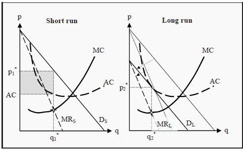
Figure 15.1: Equilibrium in the Short and Long Run for Monopolistic Competition

How far do they shift? They shift until there is no profit. Remember that, the firms choose the quantity that maximizes profit, i.e. the quantity that makes MC = MR. The demand curve, DL, will consequently shift until the quantity where the firm maximizes its profit, q2 *, is such that the price the firm can take for the good, p2*, is exactly equal to the average cost, AC. At that point, the profit is q2 *(p2* - AC) = 0.

Note that the production is not efficient. Even in the long run we have that p > MC, which means that the cost of producing additional goods is lower than the consumers’ valuations. If we compare to the results for perfect competition in the long run (see Section: Long-Run Production), we see that one difference is that long-run production in the case of monopolistic competition does not end up at the lowest point of the AC curve. This, in turn, means that there are unexploited economies of scale (compare to Section: The Relation between Long-Run and Short-Run Average Costs ). Had we had fewer firms in the market, and thereby larger firms to satisfy the demand, they would have come closer to the lowest point on the AC curve. On the other hand, we would then have had fewer (close substitute) products between which to choose. It is not possible, without a more detailed analysis, to say what balance between these two – lower unit costs or more products to choose from – that is the best for the consumers.