Labor

The labor market represents one of the most fundamental exchanges in any economy: workers selling their time and skills to firms that need labor to produce goods and services. Understanding how labor markets function is essential for economists, business leaders, and policymakers alike. This article examines the mechanics of labor supply and demand, along with how different market structures impact wages, employment levels, and economic efficiency.

The Supply of Labor: When Workers Choose Between Work and Leisure

At its core, the labor supply depends on workers' valuations of two key factors: leisure time and wages. Unlike typical goods, the supply of labor involves individuals making trade-offs with their limited time—24 hours in a day sets a natural upper limit on how much labor any person can supply.

The Worker's Perspective: Demand for Leisure

To better understand labor supply, economists often reframe the question in terms of demand for leisure. Since a person can either work or enjoy leisure time, their supply of labor equals 24 hours minus their chosen amount of leisure.

This approach allows us to apply standard consumer choice theory, where individuals maximize utility by selecting their optimal combination of leisure time and consumption goods (purchased with wages).

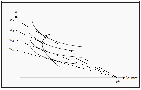
Figure 1: The Individual’s Supply of Labor

The Backward-Bending Supply Curve Phenomenon

One of the most interesting characteristics of labor supply is the backward-bending supply curve. At low wage levels, an increase in wages typically leads to an increase in labor supplied—workers sacrifice leisure to earn more. This occurs because the substitution effect (where higher wages make work more attractive relative to leisure) outweighs the income effect (where higher wages make workers wealthier and able to "purchase" more leisure).

However, as wages continue to rise, something remarkable happens: at some point, the income effect begins to dominate the substitution effect. Well-paid individuals who receive further wage increases may actually choose to work less, using their higher income to "buy back" their time in the form of more leisure. This phenomenon creates the distinctive backward-bending shape of the labor supply curve at higher wage levels.

The Demand for Labor: How Firms Value Workers

From a firm's perspective, the decision to hire workers depends on the contribution each worker makes to the firm's profit. Firms compare the cost of labor (wages) with the revenue generated by that labor.

Marginal Revenue Product of Labor (MRPL)

The key concept in labor demand is the Marginal Revenue Product of Labor (MRPL), which represents the additional revenue a firm earns by employing one more unit of labor. Mathematically:

MRPL = MR × MPL

Where:

• MR is the Marginal Revenue (the additional revenue from selling one more unit of output)
• MPL is the Marginal Product of Labor (the additional output produced by one more unit of labor)

In other words, the value of an additional worker to a firm equals how many additional units of goods that worker can produce (MPL) multiplied by the revenue the firm receives for each additional unit sold (MR).

Here, MRPL, is the marginal revenue product of labor. It corresponds to how much total revenue, TR, changes because of a small increase in L. In the third step above, we have divided and multiplied by Δq in order to show that MRPL = MR*MPL. In other words, if we hire one more unit of labor, the value-added is how many additional units of the good is produced during that hour (MPL) times at which price can we sell each additional unit (MR). That value-added is called the marginal revenue product of labor.

The Law of Diminishing Marginal Returns

An important principle affecting labor demand is the law of diminishing marginal returns. As a firm hires more workers (while keeping other factors like capital constant), each additional worker tends to add less to production than the previous one. This causes the MPL to decline as more workers are hired, which in turn makes the MRPL (and thus the demand for labor) slope downward.

Labor Markets Under Different Competitive Conditions

The interaction between labor supply and demand varies significantly depending on the competitive structure in both the labor market and the output market where firms sell their products.

Perfect Competition in Both Input and Output Markets

In the simplest scenario, both the labor market and the product market exhibit perfect competition. Under these conditions:

1. Firms cannot influence the price (p) of their output, making marginal revenue equal to price (MR = p)
2. The value of the marginal product of labor becomes MRPL = p × MPL
3. The marginal cost of labor equals the wage (MCL = w)

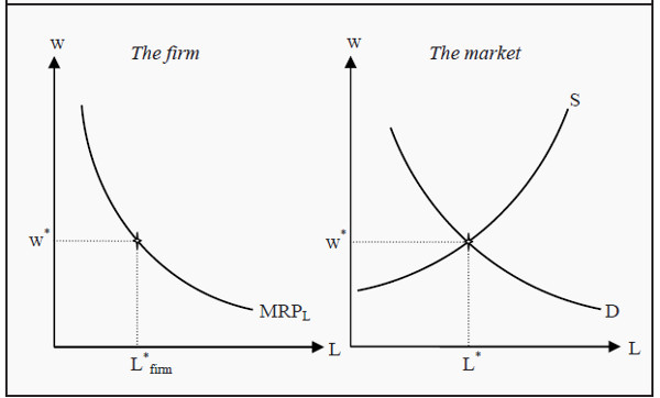
Figure 2: The Firm’s Demand for Labor and the Market Equilibrium

Profit-maximizing firms hire workers until MRPL = w, meaning they continue hiring as long as the revenue generated exceeds the cost of hiring. This makes the MRPL curve the firm's demand curve for labor.

In a perfectly competitive market equilibrium, wages are determined by the intersection of market labor supply and market labor demand (the sum of all firms' individual demand curves). This results in an efficient allocation of labor resources.

Monopoly in the Output Market

When firms sell their products in a monopolistic market while the labor market remains competitive, the analysis changes in important ways:

1. The monopolist faces a downward-sloping demand curve for its product
2. Marginal revenue (MR) is less than price and decreases with increased production
3. This makes MRPL (= MR × MPL) decrease more rapidly than in competitive markets

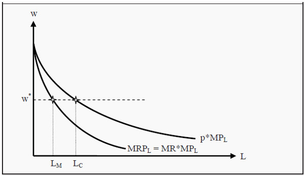
Figure 3: The Demand for Labor when the Output Market is a Monopoly

The result? A monopolist typically produces less output and therefore hires fewer workers compared to firms in competitive markets. This creates inefficiencies in both the product market and the labor market, with lower employment and output levels than would occur under perfect competition.

Monopsony in the Labor Market

A monopsony occurs when there is only one buyer in the market—in this case, a single employer hiring in the labor market. Examples might include a dominant employer in a small town or a government that employs all healthcare workers in a nationalized healthcare system.

The key insight about monopsonies is that they must raise wages for all workers to attract additional labor. This means:

1. The marginal cost of labor (MCL) exceeds the wage rate
2. The MCL curve has a steeper slope than the labor supply curve
3. The monopsonist hires workers until MRPL = MCL (not MRPL = w as in competitive markets)

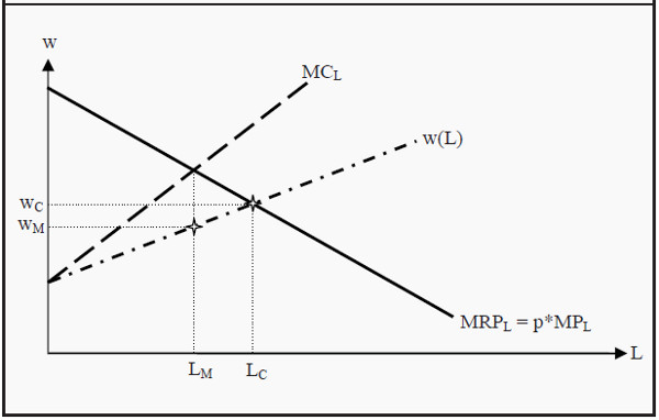
Figure 4: Monopsony

This results in lower wages and lower employment levels compared to competitive labor markets. Like monopoly in the output market, monopsony creates economic inefficiencies.

Bilateral Monopoly: When Power Meets Power

A bilateral monopoly represents a fascinating case where a monopolist (single seller) faces a monopsonist (single buyer). In labor markets, this occurs when a powerful labor union (monopoly supplier of labor) negotiates with a single employer or employer association (monopsony buyer of labor).

The outcome in bilateral monopolies depends largely on negotiation strength, economic conditions, and institutional factors. This resembles centralized wage negotiations in some countries where unions and employer organizations bargain collectively.

Practical Implications of Labor Market Structures

Understanding different labor market structures helps explain several real-world phenomena:

• Wage Disparities: Different market structures can explain why similar workers earn different wages across industries or regions.
• Policy Interventions: The effectiveness of minimum wage laws, union regulations, and other labor market policies depends on the underlying market structure.
• Employment Levels: Market structure influences hiring decisions, potentially creating inefficiencies that reduce overall employment.
• Income Distribution: The division of economic value between workers and firms varies significantly across different market structures.

Conclusion

Labor markets form a critical component of any economy, determining not only wages and employment levels but also influencing production decisions, income distribution, and economic efficiency. The complexity of labor markets stems from their dual nature—involving both the supply decisions of workers trading off leisure and wages and the demand decisions of firms maximizing profits.

Different market structures create vastly different outcomes in terms of wages, employment levels, and economic efficiency. Perfect competition tends to optimize resource allocation, while monopoly power in either the output market or the labor market (monopsony) typically reduces employment and creates inefficiencies.

For policymakers, business leaders, and workers, understanding these dynamics provides valuable insights into how labor markets function and how various interventions might affect outcomes. As labor markets continue to evolve with technological change, globalization, and shifting institutional arrangements, this understanding becomes increasingly important for navigating the complex economic landscape of the 21st century.