Keynesian cross model
- Details
- Category: Macroeconomics
- Hits: 23,615
The Keynesian model
In this chapter we will look at the Keynesian cross model. This model is a simple version of what we call the ”complete Keynesian model” or simply the Keynesian model. The Keynesian model has as its origin the writings of John Maynard Keynes in the 1930s, particularly the book ”The general theory of Employment, Interest, and Money”.
Although this book was written as a criticism of the classical model, the similarities between the Keynesian model and the classical model are definitely greater than the differences.
Lets point out the three most important differences directly:
- Say's Law does not apply in the Keynesian model.
- The quantity theory of money does not apply in the Keynesian model.
- The nominal wage level W is an exogenous variable in the Keynesian model.
Remember that W being exogenous means that it is pre-determined outside the model. It does not necessarily mean that it is constant over time – even though this is a common assumption. However,the nominal wage must be known at any point in time in this model. To simplify our description of theKeynesian model, we will begin by assuming that W is constant.
The Keynesian model is slightly more complicated than the classic model, and it is developed in four stages by analyzing four separate models. Each model has, however, a value in itself. The models we will consider and the major characteristics of each are:
- Cross model: W, P and R are constant (and exogenous).
- IS-LM model: W, P are constant and R is endogenous.
- AS-AD model: W is constant, P and R are endogenous.
- The full Keynesian model: W is exogenous (but not constant), P and R are endogenous.
Once we have developed the full Keynesian model, we will combine it with the clasmodel which will lead to the neoclassical synthesis. The final chapter covers the Mundell-Fleming model – an extension of the neoclassical synthesis to an open economy where we also analyze the exchange rate.
Summary of the cross model
The following list summarizes the cross model and relates it to the classical model:
Labor Market : The real wages W/P is exogenous in the cross model (W is exogenous in all the Keynesian models and P is exogenous in cross model). The detrmination of L is very different from the classical model, see Section Determination of L in the cross model.
Aggregate supply Ys is determined by the production function Ys = f(L, K). Again, we always remove any trend in GDP and its components.
Aggregate demand is not always equal to the aggregate supply. Say's Law does not apply in any of the Keynesian models. Therefore, we must describe how aggregate demand and GDP is determined in the cross model. This can be found in Section Determination of GDP in the cross model
The Quantity theory of money does not apply anymore. Fortunatelly, we don’t need it since P is given in the cross model.
Consumption was a function of the real interest rate in the classical model. In the cross model it is a function of Y.
Investment was also a function of r in the classical model. In the Keynesian model it is exogenous.
Government spending (G) is exogenous but the net tax NX is endogenous (in the classical model, they were both exogenous). Net tax is assumed to be a function of Y which means that government savings will be endogenous:
SG(Y )= NT(Y) – G
Exports (X) is exogenous, as it is in the classical model, but imports (Im) is endogenous.
Imports will also be a function of Y. Net imports and external savings will therefore also be endogenous variables:
NX(Y) = X – Im(Y) and SR(Y) = Im (Y) – X
Household savings and total savings were functions of the real interest rate in the classical model. In the cross model they are functions of Y.
The real interest rate is exogenous in cross model. This follows by the fact that the nominal interest rate is exogenous and prices are constant (π e must be zero, and r = R).
We can divide our analysis of the cross model into three parts:
- Aggregate demand . Aggregate demand is a major component of the cross model. The main purpose of this section is to arrive at the conclusion that aggregate demand depends on real GDP.
- Determination of GDP . GDP is determined very differently in the cross model compared to the classical model.
- Labor market . One of the main points of the Keynesian model is to allow for unvoluntary unemployment. In the classical model of the the labor market, we are always in equilibrium and there is no unvoluntary unemployment.
Aggregate demand
The consumption function
Consumption C(Y) depends positively on GDP in the cross model
Remember that in the classical model, consumption depends on the real interest rate. In the cross model it depends on GDP. Note that it is not possible to include r in the cross model as it is fixed. However, we need to justify the dependence of C on Y.
Consumption and GDP
At first, it might seem obvious that consumption will depend on Y. If GDP is doubled in real terms over a number of years, private consumption, government consumption and investment will also each roughly be doubled. If you draw a graph of GDP and consumption over time you see that consumption does grow by about the same rate as GDP.
However, from this reasoning, we cannot conclude that C depends on the Y because growth has been removed from our variables C and Y. We need to think of Y as a variable that varies over time around some average. Sometimes it is above the average and sometimes it is below the average but there is now upward trend. The same is true for C.
The crucial question then is whether consumption is above its average in periods when GDP is above its average and vise versa (technically, if the detrended variables are correlated over time). Keynes would have said yes, while classics would have said no.
Keynes' motivation: In good times, when Y is high (above its trend), national income is high (above it trend). Consumers will take the opportunity to buy things they otherwise cannot afford. In bad times, on the other hand, consumers simply cannot buy things they would have bought if income was higher. The classical motivation: Consumers want to smooth their consumption over time. In good times, consumers know that this is a temporary state. Instead of increasing consumption, they save and use their savings in bad times.
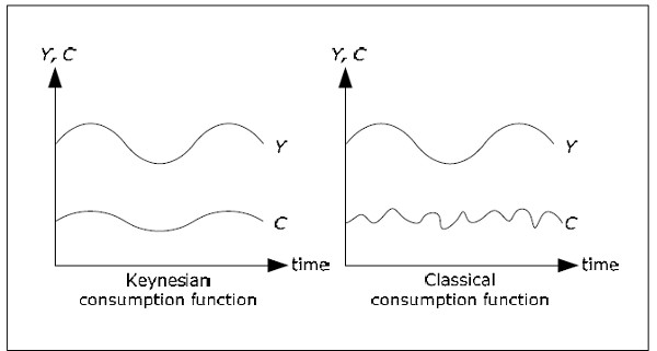
Fig. 11.1: Classical and Keynesian consumption function.
The rest of the world in the cross model
Imports Im(Y) depends positively on Y in the cross model
In the classical model, imports does not depend on Y. The discussion whether imports depends on Y or not is the same as for consumption. However, in the cross model, it is always assumed that when Y increases, consumption will increase by more than imports. This makes sense since C is usually larger than Y. For example, suppose that C is 1000 while Im is 100 and that Y increases by 10%. If C and Im increase by 5% each, C will increase by 50 while Im will increases by only 5.
Net exports NX = X – Im will depend negatively on the Y and rest of the world savings SR = Im – X depends positively on Y in the cross model. If we want to be explicit about these dependences we write:
NX (Y) = X − Im(Y)
SR (Y) = Im(Y) − X
The government in the cross model
Net taxes NT(Y) depends positively on real GDP in the cross model
In this model, when national income increases, the amount individuals pay in income taxes will increase. This is because income tax is specified as a percentage of total income. Other taxes may also increase when Y increases. However, government transfers to households will decrease . Therefore, net taxes NT will increase when Y increases.
Even though NT depends on Y, is still under the control of the government. NT may change even if Y does not change. This means that NT is part exogenous (as it may be controled by the government) and part endogenous (as it will automatically change when Y changes). Therefore, we write NT(Y) but we must remember the exogenous nature of net taxes. Government savings, which is also part endogenous and part exogenous, depends positively on Y and we write:
SG (Y) = NT(Y) − G
Savings
Household savings SH(Y) and total savings S(Y) depend positively on Y
Household savings depends on Y because SH = Y − C − NT and C and NT both depend on Y. How it depends on Y cannot be conclusively be determined from this relationship as C and NT both depends positively on Y. We always assume that this dependence is positive and the following example illustrates why this assumption makes sense.
Suppose that NT = t·Y where t is a constant between 0 and 1. t is the the proportion of income that we pay in taxes. Next, suppose that C = c·Yd where c is a constant between 0 and 1. c is proportion of disposable income that we use for consumption. If income Y increases by 1, NT increase by t, disposable income increases by 1 – t and C increases by c(1 – t). Thus, SH increases by 1 – c(1 – t) – t = (1 – c)(1 – t) > 0.
Since S = SH + SG + SR and all parts on the right hand side depends positively on Y, total saving S will depend on positive Y and we write S(Y) for total savings (net total supply of savings).
Aggregate demand in the cross model
Since C and Im depends positively on Y while G, I and X are exogenous, aggregate demand YD will depend positively on Y:
YD (Y) = C(Y) + I + G + X − Im(Y)
When Y increases, C and Im increases but since C increases more than Im, aggregate demand will increase when Y increases.
You may react to the the notation YD(Y). But if you think of Y as the national income (GDP = national income) then YD( Y) simply tells us that aggregate demand depends on income. Aggregate demand is the total quantity of finished goods and services that all sectors (consumers, firms, government and the rest of the world) together wish to buy under different conditions. The notation YD(Y) tells us that the only endogenous variable that affects aggregate demand is national income. The higher the income, the more we wish to buy. YD, C, Im, S, SH, SG, SR and NT all depend on Y while I, G and X are exogenous. We can illustrate this using the following diagrams.
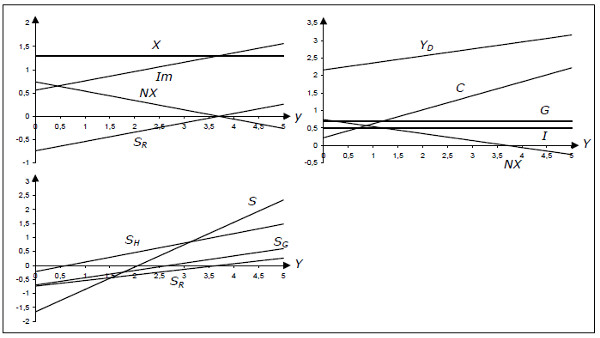
Fig. 11.2: Aggregate demand and its components.
Each diagram has real GDP on the x-axis.
- The first diagram shows exports (X), imports (Im), net exports (NX) and rest of the world savings (SR). In this diagram, X = 1.3 and Im = 0.56 + 0.2Y.
- The second diagram shows private consumption (C), investment (I), government spending (G), net exports (NX) andaggregate demand (YD = C + I + G + NX). Here, C = 0.22 + 0.4Y, I = 0.5, G = 0.7.
- The third diagram shows private savings (SH), public savings (SG), the rest of the world savings (SR) and the total savings (S = SH + SG + SR). They are created from NT = 0.26Y.
This diagram summarizes all varaiables in the cross model and how they depend on Y. Actually, these dependences will be the same in all of the Keynesian models.
Determination of GDP in the cross model
Main result
In the cross model, GDP is determined as the solution to the equation YD(Y) = Y
We may illustrate the determination of Y graphically:
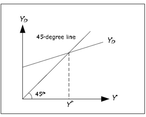
Fig. 11.3: Determination of GDP in cross model.
All points on the 45-degree line has the same x- and y-coordinates. Since we have Y on the x-axis, and YD on the y-axis, YD = Y for all points on the 45-degree line. The AD curve shows the aggregate demand YD as a function of Y. There is only one level of Y where aggregate demand is equal to Y, thepoint where AD cutts the 45-degree line. This level is called the equilibrium level of GDP and it is denoted by Y*. Formally, Y* is defined implicitly by YD(Y*) = Y*.
Justification
Note that we have not said anything about the aggregate supply so far. In order to justify why GDP is determined solely by aggregate demand we have to explain why aggregate supply YS plays no role andwhy YS always will be exactly equal to YD (which is required for the goods market to be in equilibrium).
We can explain why YS = Y* by analyzing what would happen if firms did not supply this quantity.
- Imagine that the firms supplied and also produced a larger quantity so that Y > Y*.
- From the diagram above, YD < Y and firms cannot sell everything they produce.
- Unplanned stock investments will increase by Y − YD when companies are forced to put unsold products in stock.
- Firms will then want to lower their supply. The reduction will continue until YS = Y*.
- If, on the other hand, they supply and produce too little, Y < Y* and then Yd > Y.
Stocks will now be reduced and firms will want to increase the supply. Note that the Keynesian model always assumes quantity adjustment to get back to equilibrium. There are no price adjustments in the Keynesian model.
Say's Law
Also note how the entire outcome of the cross model depends on the elimination of Say's Law. With Say's Law, aggregate demand would always be equal to aggregate supply and the cross model would be incorrect.
Keynes's argument as to why Say's Law does not apply can be illustrated in the cross model. According to Say's law, supply creates its own demand. When supply increases, income increases and a higher income creates an equally large increase in demand. Households and firms are stimulated to a higher demand by cuts in the real interest rates.
Higher aggregate supply will lower the real interest rate and consumption and investment will increase. According to Say's Law, r will fall to the level where the total increase in C and I is exactly as large as the increase in aggregate supply.
According to Keynes and cross model, this will not happen. When Y increases, C will increase but not as much as Y (and I will not change at all). Aggregate demand will not increase as much as aggregate supply and Say's Law will fail.
Reversed Say's Law
In the cross model, supply must instead follow demand. The cross model not only rejects Say's Law, it turns it completely upside down. In the cross model "demand creates its own supply".
Just as Say's Law is criticized by many economists, there is criticism of this reversed form of Say's Law. In this reversed form, firms passively produce exactly what the consumers want. If there is an increase in demand, firms will just produce this additional quantity. The motivation for this behaviour by the firms is further analyzed when we describe the labor market in the cross model.
Determination of other variables
Once Y is determined, almost all of the other variables are determined because they are either exogenous or they depend on Y. From Y we can determine C by the consumption function, Im from the import function and NT from the net tax function.
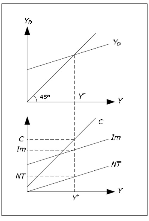
Fig. 11.4: Determination of C, Im and NT.
When these variables are determined, we can determine net exports, household savings, government savings and rest of the world savings. All macro variables except L and U are thus determined.
Labor market
Labor supply and labor demand in the Keynesian model
Remember that the supply of labor, LS(W/P), depends positively on real wages in the classical model. It is not always clear which individuals are included in the labor supply. The labor supply may consist of only individuals in the workforce or it may have a wider definition including individuals that are outside the labor force but would like to work if they could find a job. The second category may contain so-called "discouraged workers" and individuals that are in school but who would rather work.
The Keynesian labor supply differs from the classic labor supply in that it includes individulas that are outside the workforce. Therefore, for a given real wage, the Keynesian labor supply is larger than the classic labor supply. However, the Keynesian labour supply is still a positive function of the real wage.
The demand for labor LD(W/P) is the same as for the classical model. It is derived from the marginal product of profit maximizing firms. The following graph shows the classical labor supply, the Keynesian labor supply and the labor demand.
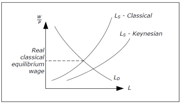
Fig. 11.5: Classical and Keynesian labor supply.
Note that for the classical equilibrium real wage, the Keynesian supply exceeds the demand. In the Keynesian models , we do not assume that the real wage will be equal to the equilibrium real wage. The labor market need not be in equilibrium in the classical sense. However, in the Keynesian models, the real wage is such that there is always an excess supply of labor (using the Keynesian supply).
The labor in the cross model
In the cross model, both P and W are constant and exogenous. Therefore, the real wage is constant and it is not necessarily equal to the equilibrium real wage. The modle of the labor market in the cross model can be illustrated by the following figure:
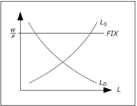
Fig. 11.6: The labor market in the cross model
Aggregate supply
Remember that labor demand gives us the profit-maximizing quantity of L for a given real wage. If W/P is given (as it is in cross model), we can find the profit-maximizing quantity of L from the graph. We denote this by LOPT. If firms use LOPT amount of labor, they wil produce YOPT = f(LOPT, K) where f is the production function and K the amount of capital (exogenous).
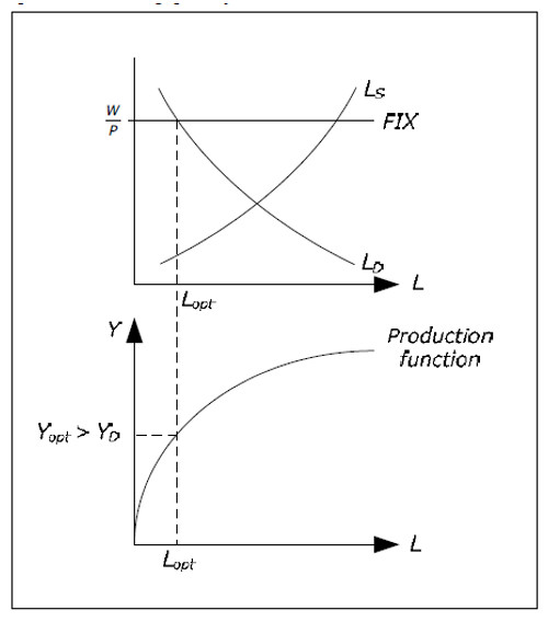
Fig. 11.7: profit-maximizing quantity of L and Y.
An important assumption in the cross model is that Y OPT is always larger than YD – the aggregate demand is not sufficient for the amount that firms would like to supply at the given real wage. This assumption has a very important consequence.
Even though producing YOPT would maximize profits,firms will not produce this level due to the lack of demand. They will only produce YD and we see why it isaggregate demand that is important in the cross model. Again, note how the Keynesian cross model works with quantity adjustments instead of price adjustments as in the classical model. We denote the level of output produced by the firms by Y*.
Determination of L in the cross model
Since firms will produce less than YOPT, they need less labor than LOPT. We can figure out exactly how much L they need in order to produce Y* and this level of L is denoted by L*.
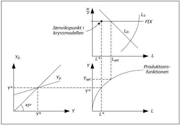
Fig. 11.8: Determination of L in the cross model.
- Start at the bottom left. Here, the equilibrium level of GDP (denoted by Y*) is determined. We can add Y* on the y-axis as well since YD = Y* in equilibrium.
- Extend Y* to the bottom-right graph. This is the aggregate supply.
- From the production function we can figure out exactly how much labor we need to produce Y*. This amount is denoted by L*.
- Extend L* up to the upper right-hand graph. Since real wage is fixed, we must be on the horizontal line and we find the equilibrium for the labor market.
- In the same diagram you will also find also find LOPT, the quantity of labor firms would choose if aggregate demand was sufficient.
Note a crucial difference between the classical and the Keynesian model: in the classical model we first determine L and go from L to Y while in the cross model we go from Y to L.
Equilibrium analysis
An important question is whether the equilibrium we have identified in the labor market (with a high unemployment rate) can remain in the long run. Will there not be adjustments that will take us back toa point with no unemployment? The Keynesian justification for why unemployment will persist is as follows.
The goods market is in equilibrium since firms will sell everything they produce and the demand for finished goods is satisfied. Firms then have no reason to hire more labor (they will only increase L when YD increases). And since the goods market is in equilibrium, they have no reason to change prices.
However, we have involuntary unemployment in the diagram above which may create a downward pressure on wages. In the cross model, this will not happen for the following arguments:
- Nominal wages are sticky, particularly downwards. We hardly ever observe cuts in nominal wages.
- Nominal wage cuts would not help. With lower wages, income would fall, reducing aggregate demand even more, making the situation worse. Lower nominal wages would allow firms to lower prices. But if prices fall as much as nominal wages, real wages will no, and we had stayed in the same paragraph.
As with the classical model, we study most of the check model characteristics in an exercise book. A couple of comments, however, may be of interest already here.
- It is difficult to explain long periods of high unemployment in the classic model with the model of labor used there.
- During the Great Depression in the early 1930s (the great depression), it became increasingly evident that the traditional model had flaws. Unemployment was very high for a long time and any adjustment to the balance of the labor market was not.
- In the Keynesian model, can the economy to be in balance even with a high level of involuntary unemployment and the model appeared to be a good explanation for depression.
- I check the model, financial policy is a very important role. By increasing G so, the government can increase GDP and thus reduce unemployment.
- The classic dichotomy between real and nominal variables will disappear in all Keynesian models.