The classical model
- Details
- Category: Macroeconomics
- Hits: 23,709
The classical model was a term coined by Keynes in the 1930s to represent basically all the ideas of economics as they apply to the macroeconomy starting with Adam Smith in the 1700s all the way up to the writings of Arthur Pigou in the 1930s.
In this chapter I will describe the main characteristics of what we now call the classical model and how the macroeconomic variables are determined in this model. As discussed in the previous section, we focus on the cycles and all the components included in the GDP (consumption, investment, imports and exports) are variables where the trend has been removed.
The classical model in this chapter will not discuss the determination of the exchange rate. In chapter 16 we will look at an extension of the classical model which will also include the exchange rate.
Labor Market
We begin by describing the classical model of the labor market.
Demand for labor
The demand for labor LD is assumed to be inversely related to the real wage W/P
Profit-maximizing firms will want to employ labor up to the point where the marginal product of labor MPL is equal to the real wage W/P. We have previously assumed that MPL is decreasing in L and the demand for labor can be illustrated in the following graph.
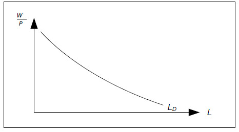
Fig. 10.1: The demand for labor.
From the graph you can conclude that the aggregate demand for labor, or just the demand for labor depends on the real wage. If the real wage increases, the demand for labor decreases and vice versa. For example, the demand for labor will fall if W increases and/or if P decreases but it will not change if W and P increase by the same percentage.
In the classical model, markets are characterized by perfect competition and the firms cannot affect W and P. However, they do decide how much labor to hire. If you sum all the labor that firms want to hire you to get the total demand for labor.
The supply of labor
The supply of labour LS is assumed to be positively related to the real wage W/P
The total labor supply is determined by utility-maximizing individuals. The total labor supply is also affected by the real wage. An increase in the real wage has two effects:
- Income Effect: With a higher income, individuals will want to consume more leisure (as long as leisure is a normal good). Higher real wages will lead to lower labor supply.
- Substitution Effect: A higher real wage will make leisure relatively more expensive, causing individuals to substitute leisure for consumption. Higher real wages will lead to higher labor supply.
The overall effect of a change in real wages is the sum of the income and substitution effects. For some individuals, the substitution effect will be stronger than the income effect and they will increase the labor supply as the real wage increases and for some it will be the opposite. In the classical model it is always assumed that the aggregate labor supply increases when real wages increase (the substitution effect is stronger than the income effect).
Equilibrium in the labor market
Real wage W/P will be equal to the equilibrium real wage in the classical model
Without government intervention and trade unions, the labor market will always be in equilibrium in the classical model. This means that the real wage will be equal to the equilibrium real wage – the level of real wage which will equilibrate the labor demand and the labor supply.
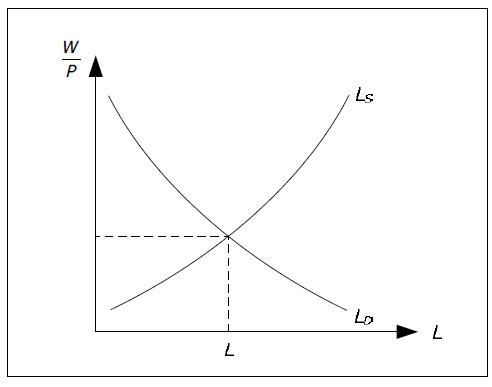
Fig. 10.2: Equilibrium in the labor market.
It is also clear from the graph that the total amount of labor L is determined in the labor market. When the real wage is equal to the equilibrium real wage, the supply of labor is equal to the demand for labor and this is the amount that will be used in the production. We then have full employment (see Wages and income).
If real wages are higher than the equilibrium real wage, the demand for labor will be less than the supply. The difference is the amount of unemployment beyond the natural rate of unemployment. In equilibrium, there is therefore no "involuntary" unemployment in the classical model.
GDP, and Say's Law
Aggregate supply
YS = f(L, K) in the classical model where
L is determined in the labor market while K is exogenous
The aggregate supply YS is defined as the amount of finished goods and services firms in a country will want to sell under given conditions. In the classical model the aggregate supply is determined by production function, YS = f(L, K).
The amount of capital in the classical model is an exogenous variable; it is not determined within the model but assumed to be given. Although we typically assume that K is constant – which is reasonable in the short run – it need not be constant. K may increase over time, but we must know K at any point in time.
The amount of labor, however, is an endogenous variable that is determined in the labor market. This means that YS is determined entirely by the labor market in the classical model. The following chart illustrates.
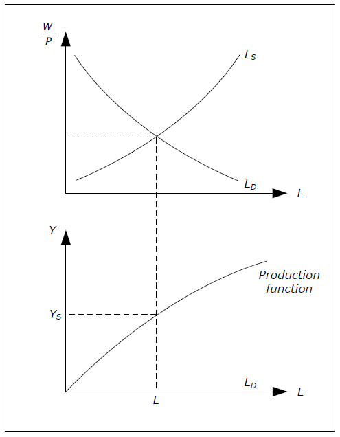
Fig. 10.3: Determination of aggregate supply.
Aggregate demand and Say's Law
YD = YS in the classical model (Say’s law)
The aggregate demand YD is defined as the quantity of nationally produced finished goods and services that consumers, government and the rest of the world want to buy under given conditions.
One of the key elements of the classical model is Say's Law. According to Say's Law the aggregate demand is always equal to the aggregate supply: YD = YS.
Say's Law is sometimes stated as "supply creates its own demand". The motivation for this statement is something like this. If production (YS) increases by one billion, the national income will also increase by one billion. This means that individuals will have exactly one more billion for spending – just enough to buy the increase in production.
Thus, YD will also increase by one1 billion. An increase in the supply of one billion has created an increase in the demand by the same amount. In the classical model, observed GDP Y will be equal to the aggregate supply: Y = YS. GDP is determined entirely by the firms and there is no need to model aggregate demand. It is always the case that YD = Y = YS = f( L, K).
How not to justify Say's Law
At first, Say's Law may seem "obvious". However, it is not – actually, it is highly controversial. The reason it may seem obvious is that you have probably learned from microeconomics that in equilibrium, demand is equal to supply. If you are outside equilibrium, prices will adjust and you will be taken back to equilibrium.
This is not the motivation behind Say's Law which is not an equilibrium condition. In the classical model, YD and YS are real variables that do not depend on the price level. This may strike you as odd. YS depends only directly on L and K and indirectly on the real wage.
If the price level increases in the classical model, the wage level will increase by the same amount leaving the real wage unchanged. As for aggregate demand, if the price level and the wage level both increase (by the same amount), there is really no change for the consumers. If all prices double while your income doubles, there is no need to adjust your demand.
The justification for Say’s Law is not an equilibrium condition through price adjustments. No price adjustment in the world will equilibrate aggregate demand and aggregate supply in the classical model. Instead, the justification is based on income effects rather than on price effects:
- higher supply
- higher income
- higher demand.
The reason why Say’s law is so controversial is the following. Suppose that consumers and investors fear that the economy will slow down. They might then decide to save a substantial part of their income and aggregate demand may not be equal to aggregate supply. This is really the starting point for Keynesian economics which we will meet in the next chapter.
The price level and the quantity theory of money
The quantity theory of money
One of the key elements of the classical model is the quantity theory of money. The quantity theory of money connects three important variables: M, P, and Y: the money supply, the price level and the real GDP.
P *Y is equal to nominal GDP. Suppose that nominal GDP is equal to 100 for a particular year while the money supply is constant and equal to 20 throughout that year. Since we are using money to buy finished goods, we may conclude that every monetary unit (USD or euro or whatever) has been used an average of 5 times during the year (100/20). This value is called the velocity of money and it is denoted by V. We have
V = (P*Y)/M
This is not a theory but a definition. What makes it into a theory – the quantity theory of money – is the assumption that V is a stable variable that does not depend on other economic variables. In the quantity theory, the velocity of money is an exogenous variable.
The quantity theory of money: M*V = P*Y, V exogenous
The main consequence of the quantity theory of money is the direct relationship between M and P if Y is constant. For example, if the money supply increases while real GDP stays the same, P will increase exactly as much as M (in percentage).
The price level
The price level is determined from the quantity theory of money:
P = (M*V)/Y
In the classical model, money supply M is an exogenous variable (hence, the growth rate in the money supply πM is exogenous). It is determined by the central bank (as discussed in the monetary base and the supply of money). Similarly V is an exogenous variable in agreement with the quantity theory of money. Thus, M*V is exogenous and given.
Remember that Y is determined by the labor market and the production function. If we combine this with the quantity theory of money, we can determine the price level P:
P = (M*V)/Y
Now, suppose that GDP is constant over time. Since V is stable (let’s say it to is constant), the percentage change in P is equal to the percentage change in M. That is, inflation is equal to the growth rate of money or π = πM.
Remember that we have removed the trend in Y which means that Y cycles around some average over time. Thus, Y is not constant over time but there is no growth in Y. Therefore, π = πM will still be approximately true even when Y is not constant (it will be true on average and in the long run).
If we do not remove the trend in Y, the result would instead be that inflation is equal to the growth in the money supply minus the growth in real GDP.
Aggregate demand
P and Y are both endogenous variables and according to the quantity theory of money we need P*Y = constant. If we divide both sides by P we get Y = constant / P. Since Y = YD in the classical model, we can write YD = constant / P. This relationship is sometimes called classical aggregate demand as it relates the real aggregate demand for goods and services YD to the price level P.
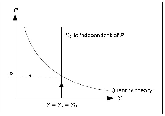
Fig. 10.4: Determination of price level.
However, it is important to remember that it is not price adjustments that make aggregate demand equal to aggregate supply in the chart above. Aggregate demand is always equal to the aggregate supply by Say's Law. In the classical model, YD is not determined by P but rather the opposite; P is determined by YD (which is equal to YS) and the money supply (which is included in the constant).
Nominal wages
W = (W/P)*P
The nominal wage is equal to the real wage times the price level.
Since the real wages, W/P is determined in the labor market and P is determined by the quantity theory of money, we can also determine the nominal wage in the classical model:
W = (W/P)P.
From the labor market, Say's Law and the quantity theory, we have now determined W, P, Y and L. We can also demonstrate how all these four are determined simultaneously:
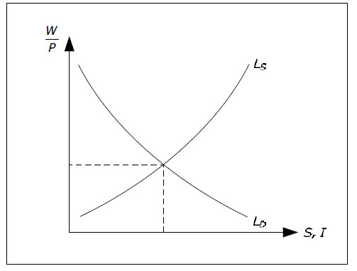
Fig. 10.5: Determination of W, P, Y and L.
Interest rate, consumption and investment
The consumption function
Consumption C(r) is assumed to be negatively related to the real interest rate r
The aggregate demand for consumer goods is defined as the total amount of finished goods and services that households wish to buy under different conditions. There is no specific supply of consumer goods – firms offer final goods but do not distinguish between the supply to consumers, the supply to investors and the supply to foreigners.
We have used the symbol C for the observed consumption. To be consistent with the notation we should denote the demand for consumer goods by CD. However, this is not common practice in macroeconomics. Instead, the symbol C is used for the demand for consumer goods as well.
Fortunately, it is almost always obvious from the context if the symbol C represents the observed consumption – it is then a variable – and when C represents the demand for consumer goods – it is then a function.
Moreover, the term “demand for consumer goods" is often shortened to the "demand for consumption" or simply "consumption". Whenever you see “consumption”, you need to figure out if it means observed consumption or consumption demand.
In the classical model, the demand for consumption is assumed to be negatively related to the real interest rate r. Higher real interest rates make it more expensive to borrow money for consumption today. Similarly, it will be more favorable to postpone consumption to the future.
Consumption is therefore denoted by C(r) and this notation makes it clear that we are talking about demand for consumption and not observed consumption.
Investment demand
Investment I(r) is assumed to be negatively related to the real interest rate r
The total demand for investment goods is defined as the total amount of investment goods firms wish to purchase under different conditions. Again, as for consumption, there is no “investment supply” and we often use “Investments” as short for the demand for investment. We use the same symbol I for observed investments and for the demand for investments.
In the classical model, investments are also negatively related to real interest r. Investments will lead to a higher income in the future and with a higher real interest rate, such future income is worthless today. Fewer projects requiring investments will be profitable and investments will decline. Investments are denoted by I(r) in the classical model.
Government revenue, government spending and net exports G, NT and NX are exogenous variables in the classical model
In the classical model (and in most macroeconomic models) government spending and net taxes are assumed to be exogenous variables determined by the government. Net Exports NX is also an exogenous variable which means that both imports Im and exports X are exogenous variables.
Exports are determined by the rest of the world and this variable is exogenous in most macro models. It is possible to assume that imports depend on the real interest rate by the same arguments we used for consumption. It would be possible to modify the classical model such that imports depended on the real interest rate but the results would be largely the same. Therefore, we assume that imports are exogenous as well.
Household savings
Remember that consumption may refer to the observed consumption as well as to the demand for consumption. The same is true for “household savings”, which may be the observed household savings as well as the supply of savings by the household sector. The supply of savings by the household sector is defined as the net amount that all households together which to lend under different conditions.
First note that for savings, we are always interested in the net. Some individuals will want to borrow and some will want to lend and some will want to do both. Household savings is the sum of all items where lending is defined as positive amounts and borrowing as negative amounts. If you borrow money in the bank, you are in effect reducing the total amounts of savings.
In the classical model the supply of savings SH depends positively on the real interest rate in the classical model. This follows by the fact that C depends negatively on r. When r increases, we consume less and save more. Therefore, household savings is denoted by SH(r).
Total savings
Total savings S(r) depends positively on the real interest rate.
Remember that total savings is defined as
S = SH + SG + SR
The sum of net savings from the household, the government and the rest of the world. As with SH, S may be the observed amount of savings or the total supply of savings. In the classical model, SG and SR are exogenous variables.
SG = NT – G and SR = Im – X
It depends only on exogenous variables and are therefore themselves exogenous.
The only part of the savings that is endogenous is household savings. Since household savings depend positively on the real interest rate, total savings will depend positively on the real interest rate. In the classical model we use S(r) to denote total savings and we have
S(r) = SH(r) + SG + SR .
Note that SH, SG, and/or SR may very well be negative. For example, when SG is negative, G > NT and the government is a net borrower.
Interest rate determination
The real interest rate r will be equal to the equilibrium real interest rate
In the classical model we define the equilibrium real interest rate r* as the real interest rate where savings is equal to investments, S(r*) = I(r*). From Components of GDP we know that S = I is a requirement for the financial market to be in equilibrium.
In the classic model, the real interest rate determines the flow of funds into and from the financial market. Higher real interest rates will lead to larger flows of funds into the market (savings depends positively on r) and the smaller flows out from the market (investment depends negatively on r). The real interest rate will be such that the flows into the market are precisely equal to the flows out of the market.
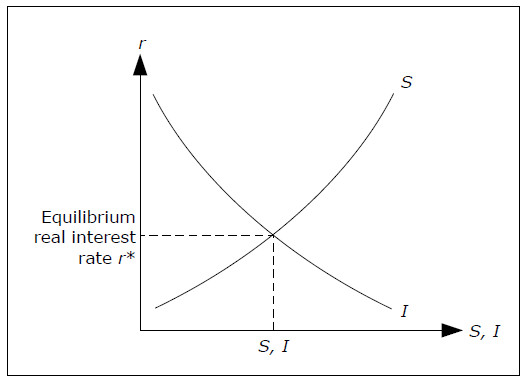
Fig. 10.6: Determination of the real rate.
From this graph we can also determine the size of investments and savings. In equilibrium when r = r*, S = I which is what we need for the GDP identity to hold. Once we know savings, we can determine household savings from
SH = S − SG − SR
In the classical model, expected inflation πe is an exogenous variable and since R = r + πe we can determine the nominal interest rate from the real rate.
Consumption
The final variable to be determined in the classical model is consumption C. Consumption may be found in several ways which will all produce exactly the same answer:
- C = C(r) from the consumption function as we know r.
- By solving for C in the equation SH = Y − NT − C. We have found Y and SH while NT is exogenous.
- By solving for C in the GDP identity Y = C + I + G + NX. We have found Y and I, while G and NX are exogenous.
Determination of all the variables in the classical model
The following diagram shows how all the variables are determined in the classical model:
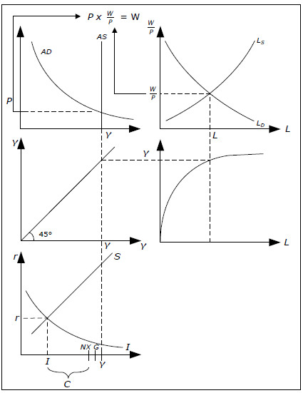
Figure 10.7 Determination of all the variables in the classical model.
- Start at the top right. Here we determine L and real wage W/P.
- Follow L down to the point on the production function in the middle to the right. Here you can find real GDP.
- Follow GDP to the left to the graph of the left in the middle. This graph consists of a single 45-degree line. All points on a 45-degree line have the same x and y coordinates. Such graph is used to transform a variable from the y axis to the x axis.
- Follow Y up to the top left graph. In this graph, you find aggregate supply which is independent of P and aggregate demand which is just the quantity theory of money. From this graph, you get up P.
- If you multiply P from the upper left-hand chart, by W/P from the upper right-hand chart, you get nominal wage W.
- Follow Y from the middle left graph down to the bottom left graph. Here is S (r) and I (r) and a determination of real r and I in the balance. In C + + NX + G = Y, and since NX and G is exogenous, we can calculate C.
We will discuss the most impact from the classical model in the exercise book, but it may be interesting to also point out here the most important:
- Monetary and fiscal policy can not affect the GDP or unemployment in the classical model.
- In the classical model can no nominal variables affect a real variable. The price level, which is a nominal variable, for example, does not affect consumption, which is a real variable. This is known as the classic dichotomy.