Long-Term Obligations

Long-Term Notes

The previous post Current Liabilities and Employer Obligations illustrations of notes were based on the assumption that the notes were of fairly short duration. Now, let’s turn our attention to longer term notes. A borrower may desire a longer term for their loan. It would not be uncommon to find two, three, five-year, and even longer term notes. These notes may evidence a term loan, where interest only is paid during the period of borrowing and the balance of the note is due at maturity.

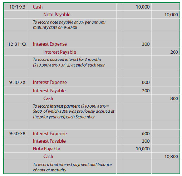
The entries are virtually the same as you saw in the previous chapter. As a refresher, assume that Wilson issued a five-year, 8% term note – with interest paid annually on September 30 of each year:

Other notes may require level payments over their terms, so that the interest and principal are fully paid by the end of their term. Such notes are very common. You may be familiar with this type of arrangement if you have financed a car or home. By the way, when you finance real estate, payment of the note is usually secured by the property being financed (if you don’t pay, the lender can foreclose on the real estate and take it over). Notes thus secured are called mortgage notes.

How do I Compute the Payment on a Note?

With the term note illustrated above, it was fairly easy to see that the interest amounted to $800 per year, and the full $10,000 balance was due at maturity. But, what if the goal is to come up with an equal annual payment that will pay all the interest and principal by the time the last payment is made? From my years of teaching, I know that students tend to perk up when this subject is covered.

It seems to be a relevant question to many people, as this is the structure typically used for automobile and real estate (mortgage) financing transactions. So, now you are about to learn how to calculate the correct amount of the payment on such a loan. The first step is to learn about future value and present value calculations.

Future Value

Let us begin by thinking about how invested money can grow with interest. What will be the future value of an investment? If you invest $1 for one year, at 10% interest per year, how much will you have at the end of the year? The answer, of course, is $1.10. This is calculated by multiplying the $1 by 10% ($1 X 10% = $0.10) and adding the $0.10 to the dollar you started with.

And, if the resulting $1.10 is invested for another year at 10%, how much will you have? The answer is $1.21. That is, $1.10 X 10% = $0.11, which is added to the $1.10 you started with. This process will continue, year after year. The annual interest each year is larger than the year before because of compounding. Compounding simply means that your investment is growing with accumulated interest, and you are earning interest on previously accrued interest that becomes part of your total investment pool. In contrast to compound interest is simple interest that does not provide for compounding, such that $1 invested for two years at 10% would only grow to $1.20.

Not to belabor the mathematics of the above observation, but you should note the following formula:

(1+i)n

Where i is the interest rate per period and n is the number of periods The formula will reveal how much an investment of $1 will grow to after n periods. For example, (1.10). = 1.21. Or, if $1 was invested for 5 years at 6%, then it would grow to about $1.34 ((1.06)5 = 1.33823). Of course, if $1,000 was invested for 5 years at 6%, it would grow to $1,338.23; this is determined by multiplying the derived factor times the amount invested at the beginning of the 5- year period.

Hopefully, you will see that it is not a great challenge to figure out how much an upfront lump sum investment can grow to become after a given number of periods at a stated interest rate. This calculation is aptly termed the future value of a lump sum amount. Future Value Tables are available that include precalculated values (the tables are found in the Appendix to this book). See if you can find the 1.33823 factor in a future value table. Likewise, use the table to determine that $5,000, invested for 10 years, at 4%, will grow to $7,401.20 ($5,000 X 1.48024).

Present Value

Present value is the opposite of future value, as it reveals how much a dollar to be received in the future is worth today. The math is simply the reciprocal of future value calculations:

1/(1+i) n

Where i is the interest rate per period and n is the number of periods For example, $1,000 to be received in 5 years, when the interest rate is 7%, is presently worth $712.99 ($1,000 X (1/(1.07)5). Stated differently, if $712.99 is invested today, it will grow to $1,000 in 5 years. Present Value Tables are available in the appendix. Use the table to find the present value of $50,000 to be received in 8 years at 8%; it is $27,013.50 ($50,000 X .54027).

Annuities

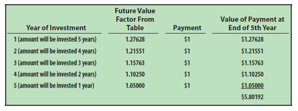
Streams of level (i.e., the same amount each period) payments occurring on regular intervals are termed annuities. For example, if you were to invest $1 at the beginning of each year at 5% per annum, after 5 years you would have $5.80. This amount can be painstakingly calculated by summing the future value amount associated with each individual payment, as shown at below.

But, it is much easier to use to an Annuity Future Value Table. The annuity table is simply the summation of individual factors. You will find the 5.80191 factor in the 5% column, 5 year row. These calculations are useful in financial planning. For example, you may wish to have a target amount accumulated by a certain age, such as with a retirement contribution account. These tables will help you calculate the amount you need to set aside each period to reach your goal. See the book Appendix for this table.

Conversely, you may be interested in an Annuity Present Value Table. This table (which is simply the summation of amounts from the lump sum present value table - with occasional rounding) shows factors that can be used to calculate the present worth of a level stream of payments to be received at the end of each period. This table is found in the Appendix to the book. Can you use the table to find the present value of $1,000 to be received at the end of each year for 5 years, if the interest rate is 8% per year, is $3,992.71? Look at the 5 year row, 8% column and you will see the 3.99271 factor.

Returning to the Original Question

How do you compute the payment on a typical loan that involves even periodic payments, with the final payment extinguishing the remaining balance due? The answer to this question is found in the present value of annuity calculations. Remember that an annuity involves a stream of level payments, just like many loans.

Now, think of the payments on a loan as a series of level payments that covers both the principal and interest. The present value of those payments is the amount you borrowed, in essence removing (discounting) out the interest component. This may still be a bit abstract, and can be further clarified with some equations. You know the following to be true for an annuity:

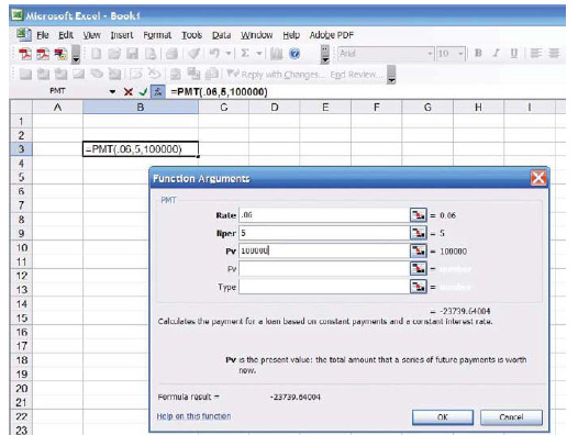
Present Value of Annuity = Payments X Annuity Present Value Factor A loan that is paid off with a series of equal payments is also an annuity, therefore: Loan Amount = Payments X Annuity Present Value Factor Thus, to determine the annual payment to satisfy a $100,000, 5-year loan at 6% per annum:

$100,000 = Payment X 4.21236 (from table)

Payment = $100,000/4.21236

Payment = $23,739.64

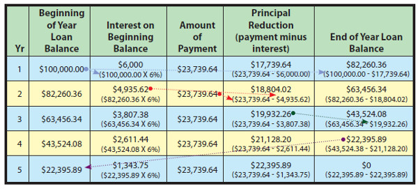
You can safely conclude that 5 payments of $23,739.64 will exactly pay off the $100,000 loan and all interest. Simply stated, the payments on a loan are just the loan amount divided by the appropriate present value factor. To fully and finally prove this point, let’s look at a typical loan amortization table. This table will show how each payment goes to pay the accumulated interest for the period, and reduce the principal, such that the final payment will pay the remaining interest and principal. You should study this table carefully:

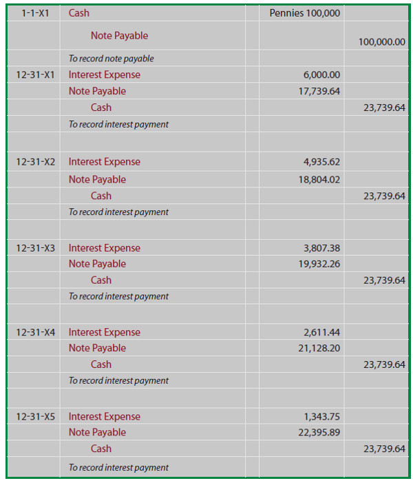
The journal entries associated with the above loan would flow as follows:

A Few Final Comments on Future and Present Value

Be very careful in performing annuity related calculations, as some scenarios may involve payments at the beginning of each period (as with the future value illustration above, and the accompanying future value tables), while other scenarios will entail end-of-period payments (as with the note illustration, and the accompanying present value table). In later chapters of this book, you will be exposed to additional future and present value tables and calculations for alternatively timed payment streams (e.g., present value of an annuity with payments at the beginning of each period).

Payments may occur on other than an annual basis. For example, a $10,000, 8% per annum loan, may involve quarterly payments over two years. The quarterly payment would be $1,365.10 ($10,000/7.32548). The 7.32548 present value factor is reflective of 8 periods (four quarters per year for two years) and 2% interest per period (8% per annum divided by four quarters per year). This type of modification does not only pertain to annuities, but also to lump sums. For example, the present value of $1 invested for five years at 10% compounded semiannually can be determined by referring to the 5% column, ten-period row.

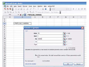
Numerous calculators include future and present value functions. If you have such a machine, you should become familiar with the specifics of its operation. Likewise, spreadsheet software normally includes embedded functions to help with fundamental present value, future value, and payment calculations. Following is a screen shot of one such routine:

Bond Payable

A borrower may split a large loan into many small units. Each of these units (or bonds) is essentially a note payable. Investors will buy these bonds, effectively making a loan to the issuing company.

Bonds were introduced, from an investor’s perspective, in the Long – term Investments chapter. The specific terms of a bond issue are specified in a bond indenture. This indenture is a written document defining the terms of the bond issue. In addition to making representations about the interest payments and life of the bond, numerous other factors must be addressed:

• Are the bonds secured by specific assets that are pledged as collateral to insure payment? If not, the bonds are said to be debenture bonds; meaning they do not have specific collateralbut are only as good as the general faith and credit of the issuer.
• What is the preference in liquidation in the event of failure? Agreements may provide thatsome bonds are paid before others.
• To whom and when is interest paid? In the past, some bonds were coupon bonds, and thesebonds literally had detachable interest coupons that could be stripped off and cashed in onspecific dates. One reason for coupon bonds was to ease the recordkeeping burden on bondissuers -- they merely paid coupons that were turned in for redemption. Coupon bonds alsohad certain tax implications that are no longer substantive. But, in modern times, mostbonds are registered to an owner. Computerized information systems now facilitate trackingbond owners, and interest payments are commonly transmitted electronically to theregistered owner. Registered bonds are in contrast to bearer bonds, where the holder of thephysical bond instrument is deemed to be the owner (bearer bonds are rare in the moderneconomic system).
• Must the company maintain a required sinking fund? A sinking fund bond may sound bad,but it is quite the opposite. In the context of bonds, a sinking fund is a required escrowaccount into which monies are periodically transferred to insure that funds will be availableat maturity to satisfy the obligation. As an alternative, some companies will issue serialbonds. Rather than the entire issue maturing at once, portions of the serial issue will matureon select dates spread over time.
• Can the bond be converted into stock? One exciting type of bond is a convertible bond.These bonds enable the holder to exchange the bond for a predefined number of shares ofcorporate stock. The holder may plan on getting paid the interest plus face amount of thebond, but if the company’s stock explodes upward in value, the holder may do much betterby trading the bonds for appreciated stock. Why would a company issue convertibles? First,investors love these securities (for obvious reasons) and are usually willing to accept lowerinterest rates than must be paid on bonds that are not convertible. Another factor is that thecompany may contemplate its stock going up; by initially borrowing money and laterexchanging the debt for stock, the company may actually get more money for its stock thanit would have had it issued the stock on the earlier date.
• Is the company able to call the debt? Callable bonds provide a company with the option ofbuying back the debt at a prearranged price before its scheduled maturity. If interest rates godown, the company may not want to be saddled with the higher cost obligations and canescape the obligation by calling the debt. Sometimes, bonds cannot be called. For example,suppose a company is in financial distress and issues high interest rate debt (known as junk bonds) to investors who are willing to take a chance to bail out the company. If thecompany is able to manage a turnaround, the investors who took the risk and bought thebonds don’t want to have their high yield stripped away with an early payoff beforescheduled maturity. Bonds that cannot be paid off earlier are sometimes callednonredeemable. If you invest in bonds, and want to buy nonredeemable debt, be careful notto confuse it with nonrefundable. Nonrefundable bonds can be paid off early, so long as thepayoff money is coming from operations rather than an alternative borrowing arrangement.Lastly, you should note that convertible bonds will almost always be callable, enabling the company to force a holder to either cash out or convert. The company will reserve this call privilege because they will want to stop paying interest (by forcing the holder out of the debt) once the stock has gone up enough to know that a conversion is inevitable.

Your head is probably spinning with all these new terms, and you can see that bonds are potentially complex financial instruments. Who enforces all of the requirements for a company’s bond issue? Within the bond indenture agreement should be a specified bond trustee. This trustee may be an investment company, law firm, or other independent party. The trustee is to monitor compliance with the terms of the agreement, and has a fiduciary duty to intervene to protect the investor group if the company runs afoul of its covenants.

Accounting for Bonds Payable

Cash Flow facts 8% stated rate

A bond payable is just a promise to pay a stream of payments over time (the interest component), and a fixed amount at maturity (the face amount). Thus, it is a blend of an annuity (the interest) and lump sum payment (the face). To determine the amount an investor will pay for a bond, therefore, requires some present value computations to determine the current worth of the future payments. To illustrate, let’s assume that Schultz Company issues 5-year, 8% bonds. Bonds frequently have a $1,000 face value, and pay interest every six months. To be realistic, let’s hold to these assumptions.

Par scenario Market rate of 8%

If 8% is the market rate of interest for companies like Schultz (i.e., companies having the same perceived integrity and risk), when Schultz issues its 8% bonds, then Schultz’s bonds should sell at face value (also known as par or 100). That is to say, investors will pay $1,000 for a bond and get back $40 every six months ($80 per year, or 8% of $1,000). At maturity they will also get their $1,000 investment back. Thus, the return on the investment will equate to 8%.

Premium scenario Market rate of 6%

On the other hand, if the market rate is only 6%, then the Schultz bonds look pretty good because of their higher stated 8% interest rate. This higher rate will induce investors to pay a premium for the Schultz bonds. But, how much more will they pay? The answer to this question is that they will bid up the price to the point that the effective yield (in contrast to the stated rate of interest) drops to only equal the going market rate of 6%. Thus investors will pay more than $1,000 to gain access to the $40 interest payments every six months and the $1,000 payment at maturity. The exact amount they will pay is determined by discounting (i.e., calculating the present value) the stream of payments at the market rate of interest. This calculation is demonstrated below, followed by an additional explanation.

Discount scenario Market rate of 10%

Also, consider the alternative scenario. If the market rate is 10% when the 8% Schultz bonds are issued, then no one would want the 8% bonds unless they can be bought at a discount. How much discount would it take to get you to buy the bonds? The discount would have to be large enough so that the effective yield on the initial investment would be pushed up to 10%. That is to say, your price for the bonds would be low enough so that the $40 periodic payment and the $1,000 at maturity would give you the requisite 10% market rate of return. The exact amount is again determined by discounting (i.e., calculating the present value) the stream of payments at the market rate of interest.

The table below calculates the price under the three different assumed market rate scenarios:

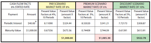
To further explain, the interest amount on the $1,000, 8% bond is $40 every six months. Since the bonds have a 5-year life, there are 10 interest payments (or periods). The periodic interest is an annuity with a 10-period duration, while the maturity value is a lump-sum payment at the end of the tenth period. The 8% market rate of interest equates to a semiannual rate of 4%, the 6% market rate scenario equates to a 3% semiannual rate, and the 10% rate is obviously 5% per semiannual period.

The present value factors are taken from the present value tables (annuity and lump-sum, respectively). You should take time to trace the factors to the appropriate tables. The present value factors are multiplied times the payment amounts, and the sum of the present value of the components would equal the price of the bond under each of the three scenarios. Note that the 8% market rate assumption produced a bond priced at $1,000, the 6% assumption produced a bond priced at $1,085.30 (which includes an $85.30 premium), and the 10% assumption produced a bond priced at $922.78 (which includes a $77.22 discount).

These calculations are not only correct theoretically, but you will find that they are very accurate financial tools -- reality will emulate theory. But, one point is noteworthy. Bond pricing is frequently done to the nearest 1/32nd. That is, a bond might trade at 103.08. You could easily misinterpret this price as $1,030.80. But, it actually means 103 and 8/32. In dollars, this would come to $1,032.50 ($1,000 X 103.25). So, now you should understand the theory and mechanics of how a bond is priced. It is time to examine the correct accounting.

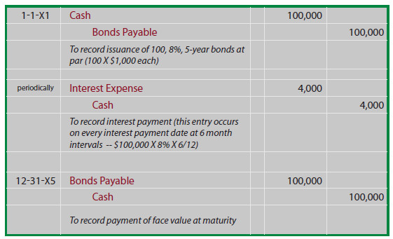
Bond Issued at Par

If Schultz issued 100 of its bonds at par, the following entries would be required, and probably require no additional explanation:

Bond Issued at Premium

You will likely need to reread this paragraph several times before it really starts to sink in. One very simple way to consider bonds issued at a premium is to reduce accounting to its simplest logic - - counting money! If Schultz issues 100 of the 8%, 5-year bonds when the market rate of interest is only 6%, then the cash received is $108,530 (see the previous discussion for the related calculations).

Schultz will have to repay a total of $140,000 ($4,000 every 6 months for 5 years, plus $100,000 at maturity). Thus, Schultz will repay $31,470 more than was borrowed ($140,000 - $108,530). This $31,470 must be expensed over the life of the bond; uniformly spreading the $31,470 over 10 six month periods produces periodic interest expense of $3,147 (do not confuse this amount with the cash payment of $4,000 that must be paid every six months!).

Another way to consider this problem is to note that total borrowing cost is reduced by the $8,530 premium, since less is to be repaid at maturity than was borrowed up front. Therefore, the $4,000 periodic interest payment is reduced by $853 of premium amortization each period ($8,530 premium amortized on a straight line basis over the 10 periods), producing the periodic interest expense of $3,147 ($4,000 - $853)!

This topic is inherently confusing, and the journal entries are actually helpful in clarifying your understanding. As you look at these entries, notice that the premium on bonds payable is carried in a separate account (unlike accounting for investments in bonds covered in a prior chapter, where the premium was simply included with the Investment in Bonds account).

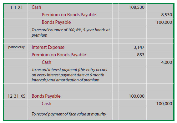
By carefully studying the following illustration you will observe that the Premium on Bonds Payable is established at $8,530, then reduced by $853 every interest date, bringing the final balance to zero at maturity.

On any given financial statement date, Bonds Payable is reported on the balance sheet as a liability, along with the unamortized Premium appended thereto (known as an adjunct account). To illustrate, the balance sheet disclosure as of 12-31-X3 would appear as follows:

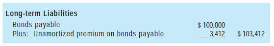
The income statement for all of 20X3 would include $6,294 of interest expense ($3,147 X 2). This method of accounting for bonds issued at a premium is known as the straight-line amortization method, as interest expense is recognized uniformly over the life of the bond. The technique offers the benefit of simplicity, but it does have one conceptual shortcoming. Notice that interest expense is the same each year, even though the net book value of the bond (bond plus remaining premium) is declining each year due to amortization.

As a result, interest expense each year is not exactly equal to the effective rate of interest (6%) that was implicit in the pricing of the bonds. For 20X1, interest expense can be seen to be roughly 5.8% of the bond liability ($6,294 expense divided by beginning of year liability of $108,530). For 20X4, interest expense is roughly 6.1% ($6,294 expense divided by beginning of year liability of $103,412). Accountants have devised a more precise approach to account for bond issues called the effective interest method. Be aware that the more theoretically correct effective interest method is actually the required method, except in those cases where the straight-line results do not differ materially. Effective-interest techniques are introduced in a following section of this chapter

Bond Issued at a Discount

If Schultz issues 100 of the 8%, 5-year bonds for $92,278 (when the market rate of interest is 10% -- see the previous discussion for exact calculations), Schultz will still have to repay a total of $140,000 ($4,000 every 6 months for 5 years, plus $100,000 at maturity). Thus, Schultz will repay $47,722 ($140,000 - $92,278) more than was borrowed. This $47,722 must be expensed over the life of the bond; spreading the $47,722 over 10 six-month periods produces periodic interest expense of $4,772.20 (do not confuse this amount with the cash payment of $4,000 that must be paid every six months!).

Another way to consider this problem is to note that the total borrowing cost is increased by the $7,722 discount, since more is to be repaid at maturity than was borrowed upfront. Therefore, the $4,000 periodic interest payment is increased by $772.20 of discount amortization each period ($7,722 discount amortized on a straight line basis over the 10 periods), producing periodic interest expense that totals $4,772.20! Now, let’s look at the entries for the bonds issued at a discount. Like bond premiums, discounts are also carried in a separate account.

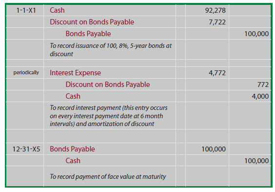
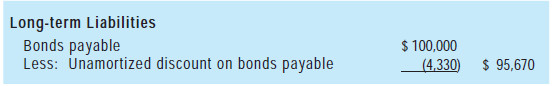
By carefully studying this illustration, you will observe that the Discount on Bonds Payable is established at $7,722, then reduced by $772.20 on every interest date, bringing the final balance to zero at maturity. On any given financial statement date, Bonds Payable is reported on the balance sheet as a liability, along with the unamortized Discount that is subtracted (known as a contra account). The illustration below shows the balance sheet disclosure as of June 30, 20X3. Note that the unamortized discount on this date is determined by calculations revealed in the table that follows:

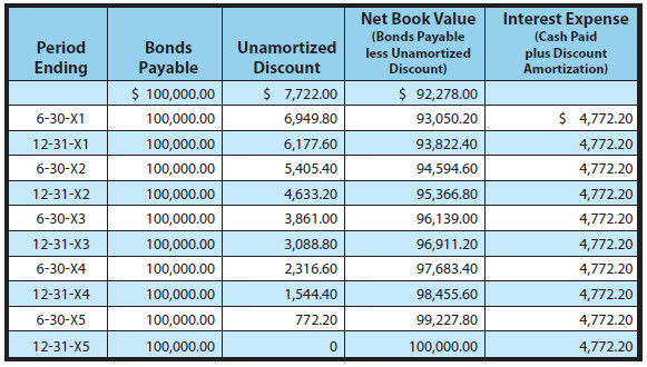
The income statement for each year would include $9,544.40 of interest expense ($4,772.20 X 2) under this straight-line approach. It again suffers from the same theoretical limitations that were discussed for the straight-line premium example. But, it is an acceptable approach if the results are not materially different from those that would result with the effective-interest amortization technique.

Affective-Interest Amortization Methods

The theoretically preferable approach to recording premium and discount amortization is the effective-interest method. It recognizes interest expense as a constant percentage of the bond’s carrying value, rather than as an equal dollar amount each year. The theoretical merit rests on the fact that the interest calculation aligns with the basis on which the bond was priced; that is to say, the interest expense is calculated as the effective-interest rate times the bond’s carrying value for each period. The amount of amortization is the difference between the cash paid for interest and the calculated amount of bond interest expense.

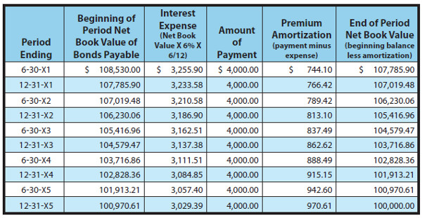
The Premium Illustration

Recall that when Schultz issued its bonds to yield 6%, it received $108,530. Thus, effective interest for the first six months is $108,530 X 6% X 6/12 = $3,255.90. Of this amount, $4,000 is paid in cash and $744.10 ($4,000 - $3,255.90) is premium amortization. The premium amortization reduces the net book value of the debt to $107,785.90 ($108,530 - $744.10). This new balance would then be used to calculate the effective interest for the next period. This process would be repeated period after period. The following table demonstrates the full amortization process for the life of Schultz’s bonds.

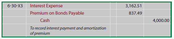
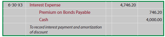
The initial journal entry to record the issuance of the bonds, and the final journal entry to record repayment at maturity would be identical to those demonstrated for the straight-line method. However, each journal entry to record the periodic interest expense recognition would vary and can be determined by reference to the above amortization table. For instance, the recording of interest on 6-30-X3 would appear as follows:

The resulting balance sheet disclosure as of June 30, 20X3, would include the following:

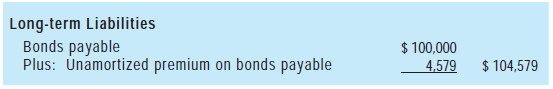
The resulting balance sheet disclosure as of June 30, 20X3, would include the following: With effective-interest techniques, interest expense varies in direct proportion to the ever reducing amount of debt. Thus, interest expense is a constant percentage of the reported debt rather than a constant amount of expense as with the straight-line method.

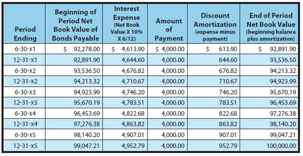
The Discount Illustration

Recall that when Schultz issued its bonds to yield 10%, it received only $92,278. Thus, effective interest for the first six months is $92,278 X 10% X 6/12 = $4,613.90. Of this amount, $4,000 is paid in cash, and $613.90 is discount amortization. The discount amortization increases the net book value of the debt to $92,891.90 ($92,278.00 + $613.90). This new balance would then be used to calculate the effective interest for the next period. This process would be repeated period after period. The following table demonstrates the full amortization process for the life of Schultz’s bonds.

be determined by reference to the above amortization table. For instance, the recording of interest on June 30, 20X3, would appear as follows:

The resulting balance sheet disclosure as of June 30, 20X3, would include the following:

Bonds Issued Between Interest Dates and Bond Retirement

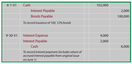
This issue is best understood in the context of a specific example. Suppose Thompson Corporation proposed to issue $100,000 of 12% bonds, dated April 1, 20X1. However, despite the April 1 date, the actual issuance was slightly delayed, and the bonds were not sold until June 1. Nevertheless, the covenant pertaining to the bonds specifies that the first 6-month interest payment date will occur on September 30 in the amount of $6,000 ($100,000 X 12% X 6/12).

In effect, interest for April and May has already accrued ($100,000 X 12% X 2/12 = $2,000) at the time the bonds are actually issued. To be fair, Thompson will collect $2,000 from the purchasers of the bonds at the time of issue, and then return it within the $6,000 payment on September 30 -- effectively causing the net difference of $4,000 to represent interest expense for June, July, August, and September ($100,000 X 12% X 4/12). The resulting journal entries are:

You should also be aware that the concepts just revealed for bonds issued between interest payment dates are also applicable to bonds that are traded between investors. There is no requirement, indeed no expectation, that bond investors will continue to hold bonds to maturity. Bonds are financial instruments that are traded between investors, just like stocks.

When bond investors sell bonds between interest dates, they will receive from the purchaser the price plus accrued interest, knowing that the purchaser will then receive a full period’s interest on the next regularly scheduled interest date. This mechanism is intended to simplify the bond issuer’s accounting by allowing one interest payment to the current holder, rather than having to provide pro-rata payments to the various investors who have held the bonds for a portion of each interest period.

Someday you will likely consider investing in bonds, and this information about the handling of accrued interest between interest dates will come in useful to you. And, you also need to be keenly aware that your bond investments can change in value.

Remember that the value of a bond is a function of the bond’s stated rate of interest in relation to the going market rate of interest. If market interest rates rise while you hold your bond investment, look for its market value to decline (reflecting a lower present value based on the higher discount rate) -- and vice versa. Of course, if you hold on to the bond to maturity, its value will converge to the face value (so long as the issuer does not go broke)!

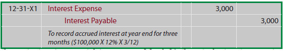
Year-end Interest Accruals

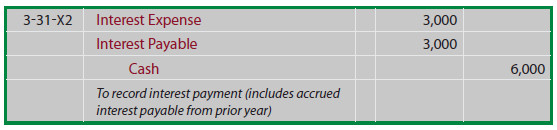
Continuing the illustration for Thompson, what December 31, 20X1, adjusting entry would be needed to bring the books current at year end? Notice that interest was paid in full through September 30. Therefore, the year-end entry must reflect the accrual of interest for October through December:

When the next interest payment date arrives on March 31, the actual interest payment will cover the previously accrued interest, and additional amounts pertaining to January, February, and March:

Any end-of-period entries would also include adjustments of interest expense for the amortization of existing bond premiums or discounts relating to the elapsed time periods.

Bonds may be Retired Before Scheduled Maturity

Early retirements of debt may occur, because a company has generated sufficient cash reserves from operations, and the company wants to stop paying interest on outstanding debt. Or, interest rates may have changed, and the company wants to take advantage of more favorable borrowing opportunities; you have probably heard of individuals engaging in this type of strategy when they refinance a home loan.

Whether the debt is being retired or refinanced in some other way, accounting rules dictate that the retired debt be removed from the books, and that the difference between the debt’s net carrying value and the funds paid to retire the debt be recognized as a gain or loss. For instance, assume that Cabano Corporation is retiring $200,000 face of its 6% bonds payable.

The last semiannual interest payment occurred on April 30, and the bonds are being retired on June 30, 20X5. The unamortized discount on the bonds at April 30, 20X5, was $6,000, and there was a 5-year remaining life on the bonds as of that date. Further, Cabano is paying $210,000, plus accrued interest, to retire the bonds; this early call price was stipulated in the original bond covenant. The first step to account for this bond retirement is to bring the accounting for interest up to date:

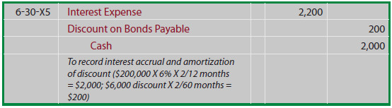
Then, the actual bond retirement can be recorded, with the difference between the up-to-date carrying value and the funds utilized being recorded as a loss (debit) or gain (credit).

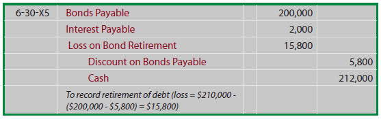
Notice that Cabano’s loss relates to the fact that it took a lot more cash ($210,000) to pay off the debt than was the debt’s carrying value ($194,200 ($200,000 minus $5,800)).

Analysis, Commitments, Alternative Financing Arrangements, Leases, and Fair Value Measurements

Careful analysis is essential in making judgments about an entity’s financial health. One form of analysis is ratio analysis where certain key metrics are evaluated against one another. One such ratio is debt to total assets. This ratio shows the percentage of total capitalization that is provided by the creditors of a business:

Debt to Total Assets Ratio = Total Debt/Total Assets

A related ratio would be debt to equity that divides total debt by total equity:

Debt to Equity Ratio = Total Debt/Total Equity

The debt to asset and debt to equity ratios are carefully monitored by investors, creditors, and analysts. The ratios are often seen as signs of financial strength when small, or signs of vulnerability when large. Of course, small and large are relative terms. Some industries, like the utilities, are inherently dependent on debt financing but may, nevertheless, be very healthy.

On the other hand, some high-tech companies may have little or no debt but be seen as vulnerable due to their intangible assets with potentially fleeting value. In short, one must be careful to correctly interpret a company’s debt related ratios. One must also be careful to recognize the signals and trends that may be revealed by careful monitoring of these ratios. Another ratio is the times interest earned ratio:

Times Interest Earned Ratio = Income Before Income Taxes and Interest/Interest Charges

This ratio is intended to demonstrate how many times over the income of the company is capable of covering its unavoidable interest obligation. If this number is relatively small, it may signal that the company is on the verge of not generating sufficient operating results to cover its mandatory interest obligation.

There are numerous other ratios that can be described; in fact, many of these are covered in other chapters (along with mathematical illustrations). However, while ratio analysis is an important part of evaluating a company’s financial health, one cannot be too careful or place undue reliance on any single evaluative measure. This will become quite apparent as you read the final concluding comments below.

Contractual Commitments and Alternative Financing Arrangements

A company may enter into a long-term agreement to buy a certain quantity of supplies from another company, agree to make periodic payments under a lease (or similar arrangement) for many years to come, agree to deliver products at fixed prices in the future, and so forth. There is effectively no limit or boundary on the nature of these commitments and agreements. Oftentimes, such situations do not result in a presently recorded obligation, but may give rise to an obligation in the future.

This introduces a myriad of accounting issues that are beyond the scope of introductory accounting courses, but a few generalizations are in order. First, footnote disclosures are generally required for the aggregate amount of committed payments that must be made in the future (with a year by year breakdown). Second, changes in the value of such commitments may entail loss recognition when a company finds itself locked into a future transaction that will have negative economic effects (e.g., committing to buy oil at $80 per barrel when the current price has declined to $65). From these observations, one thing should be clear to you -- beware to not limit your evaluation of a company to just the numbers on the balance sheet, as significant other financial details are often found in notes to the financial statements.

Capital Leases

A previous chapter introduced the idea of a capital lease. Such transactions enable the lessee to acquire needed productive assets, not by outright purchase, but by leasing. The economic substance of capital leases, in sharp contrast to their legal form, is such that the lessee effectively assumes the risks and rewards of owning the asset. Further, the accompanying obligation for lease payments is akin to a note payable.

That is, the lessee is under contract to make a stream of payments over time that substantively resembles the stream of payments that would have occurred had the lessee purchased the asset via a promissory note. Accounting rules attempt to track economic substance ahead of legal form. Thus, when an asset is acquired via a capital lease, the initial recording is to establish both the asset and related obligation on the lessee’s balance sheet.

Assume that equipment with a five-year life is leased on January 1, 20X1, and the lease agreement provides for 5 end-of-year lease payments of $23,739.64 each. At the time the lease was initiated, the lessee’s incremental borrowing rate (the interest rate the lessee would have incurred on similar debt financing) is assumed to be 6%. The accountant would discount the stream of payments using the 6% interest rate and find that the present value of the fixed non cancelable lease payments is $100,000. Therefore, the following entry would be necessary to record the lease:

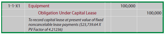
After the initial recording, the accounting for the asset and obligation take separate paths. The asset is typically depreciated over the lease term (or useful life, depending on a variety of conditions). The depreciation method might be straight-line or an accelerated approach. Essentially, the leased asset is accounted for like any other owned asset of the company. The Obligation Under Capital Lease is accounted for like a note payable. In the above example, the amounts happen to correspond to the amounts illustrated for the mortgage note introduced earlier in the chapter. Therefore, the first lease payment would be accounted for as follows:

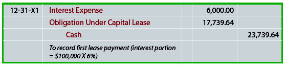
Notice that this entry results in recording interest expense - not rent. This scheme would be applied for each successive payment, until the final payment extinguishes the Obligation Under Capital Lease account. The accounting outcome is virtually identical (i.e., changing amounts of interest expense as the obligation is reduced over time) to that associated with the mortgage note illustrated earlier in the chapter.

The Fair Value Measurement Option

The Financial Accounting Standards Board recently issued a profound standard, The Fair Value Option for Financial Assets and Financial Liabilities. The title is quite revealing. Companies are now permitted, but not required, to measure certain financial liabilities at fair value. Changes in fair value can result from many factors, including market conditions pertaining to the overall interest rate environment. Entities that opt for this standard are to report unrealized gains and losses on items for which the fair value option has been elected in earnings at each subsequent reporting date.

This new standard is a profound shift in methodology, and has the potential to eventually reshape debt accounting. Because the new standard is optional and somewhat controversial, it is very difficult to predict its practical effect and eventual implications. However, it is indicative of a clear intent to embrace more fair value methodology into the overall accounting framework.