The neo-classical synthesis
- Detalii
- Categorie: Macroeconomics
- Accesări: 10,176
The neo-classical synthesis is a synthesis of the classical model and the Keynesian model. In short, it states that the Keynesian model is correct in the short run while the classical analysis is correct in the long run. Let us consider a concrete example. According to the Keynesian model, an increase in G will increase Y and reduce unemployment.
In the classical model, an increase in G will have no effect at all on Y and unemployment. In the neo-classical synthesis, an increase in G will create a temporary increase in Y but Y will return to its original value after some time.
To justify the neo-classical synthesis, it is helpful to identify the problem with the classical model in the short run and the problem with the Keynesian model in the long run. As for the classical model in the short run, we concluded that within this model, it is difficult to explain deep recessions with high involuntary unemployment. In the long run, it is more reasonable to believe that that the economy can get out of the recession by itself. The problem with the Keynesian model in the long run, as we will see, is the assumption of a stable Phillips curve.
The various Phillips curves
The augmented Phillips curve
Remember that the Phillips curve, as it was incorporated into the Keynesian model, assumed a stable relationship between unemployment and wage inflation: for a given level of unemployment (say U = 5%), a given level of wage inflation would apply (say πw = 4%). As U increased, π w would fall and vice versa.
Mathematically, the Phillips curve may be described by a decreasing function f as:
πw = f(U)
In the neo-classical synthesis, expected inflation is added and:
πw = f(U) + πe
To justify this amendment, imagine U = 5% and πw = 4% (so that we are on the Phillips curve) and the expected inflation rises from 4% to 6%. Since employees care about real wages, it is reasonable to assume that πw will increases as well (for a given U) and the Phillips curve will shift upwards.
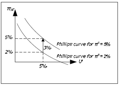
Fig. 15.1: The augmented Phillips curve.
According to the synthesis, the Phillips curve must be drawn for a given value of πe and it must be shifted upwards (downwards) as πe increases (decreases). When the position of the Phillips curve is allowed to depend on πe, is called the augmented Phillips curve (or the expectations-augmented Phillips curve). This amendment to the Phillips curve is actually a consequence of a criticism of the traditional Phillips curve and the Keynesian model from the late 1960's (the Keynesian – Monetarism debate).
Money illusion
An important argument for the augmentation has to do with the concept of money illusion. Money illusion means that you care about nominal rather than real amounts. Imagine that your salary
increases by 20% over one year. Does this mean that you can increase your consumption? The answer is that it depends on the inflation. If inflation is 20%, you can consume as much as you did before. You must actually decrease you consumption if inflation exceeds 20%. We say that you have suffer from money illusion if you believe that you are better off if your salary increases by 20% while prices also increase by 20%. A higher nominal salary may create the "illusion" that you are richer.
If employees suffer from money illusion they will only care about nominal wage increases, expected inflation will not matter and there is no reason for the traditional Phillips curve not to hold. If, however, they do not suffer from money illusion, πw must depend on both U and πe and the augmented Phillips curve is more realistic.
The long-run Phillips curve
The augmented Phillips curve has an important consequence: the long-run Phillips curve must be vertical.
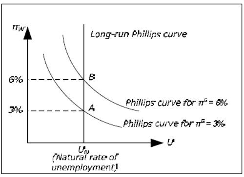
Fig. 15.2: The long-term Phillips curve.
To realize this, start by drawing a Phillips curve for πe = 3%. The only point on this curve that may apply in the long run is π W = 3% (point A). For example, πW = 2% and πe = 3% is not consistent with equilibrium in the long run as there is no level of inflation which is consistent with these values. π = 3% is not possible as real wages would go to zero. π = 2% is not possible since it would be unreasonable to continue to expect 3% inflation if inflation each year was 2%.
According to the neo-classical synthesis, we may temporarily be anywhere on the lower Phillips curve when πe = 3%, but the economy must eventually return to point A (as long πe = 3%) Now draw a Phillips curve for πe = 6%. Again, on this curve there is only one point is consistent with equilibrium in the long run and that is the point where πW = 6% (point B). This point must be exactly above A as the new curve must be exactly three units above the first curve.
If we draw all possible Phillips curves, we see that all points consistent with long run equilibrium must lie on a vertical curve and this curve is called the long-run Phillips curve. In the long run, the economy must return to this curve. This means that in the long run, there is no relation between inflation and unemployment. In the long term, the economy returns to the natural unemployment rate as in the classical model.
Summary of the Phillips curves
In the neo-classical synthesis, the augmented Phillips curve is called the short-run Phillips curve. It is assumed to be stable as long as expectations of future inflation do not change. To summarize, we have three Phillips curves:
- The traditional Phillips curve. πW = f(U) and the same downward sloping relationship applies to both the short and the long run.
- The short-run Phillips curve (SPC). πw = f(U) + πe and the curve is valid only in the short run (SPC = Short-run Phillips Curve).
- The long-run Phillips curve (LPC). πw = πM, U = UN and there is no relationship between πwand U (UN is the natural rate of unemployment).
The classical model and the long-term Phillips curve
In the classical model, L and the real wage are determined from equilibrium conditions in the labor market. L and W / P , therefore, are only affected by the marginal product of labor (which determines the demand for labor) and by the utility function of the employees (which determines the supply of labor). All unemployment is voluntary and L, U or W / P are all affected by exogenous variables only.
In the classical model, inflation is determined solely by the growth in the money upply πM. From the quantity theory of money, M·V = P·Y and if the growth rate of M is πM, then P must increase by the same rate as V and Y are constant. From the quantity theory we can conclude that π = πM must hold.
The relationship M·V = P·Y is therefore sometimes called the quantity theory in levels while π = πM is called the quantity theory in rates. In the classical model, inflation is balanced and πW = π (real wage is constant). Since π = π M, we have π = πM = πW. As U is not affected by any endogenous variables, there is no relationship between πW
och U in the classical model and the vertical LPC applies even in the short run. The position on the LPC determined by πM.
Unlike the neo-classical synthesis, where the economy temporarily may depart from LPC, the economy must always be on the LPC in the classical model.
Developments around 1960
The augmented Phillips curve and the long-run Phillips curve where developed during the late 1960s by Milton Friedman and Edmund Phelps. Friedman argued that a stable Phillips curve could exist in the short run as long individuals did not expect changes in the economy. Eventually, expectations would change and the traditional Phillips curve would shift and we would return to a point on the long-run Phillips curve.
If the Phillips curve depends on πe, we can no longer expect observations of nemployment and wage inflation to nicely line up on a downward sloping curve. Instead, different observations will belong to different Phillips curves that move over time and we should expect to see all possible combinations of U och πw.
Most Keynesian chose to hold on to the traditional Phillips curve. If you buy the augmented Phillips curve, you must buy the long-run Phillips curve and the economy must automatically return to the natural level of unemployment. This would violate one of the main results in the Keynesian analysis namely that the economy may be stuck in a long-run equilibrium with a high level of involuntary unemployment. With the long-run Phillips curve, it would again be impossible to determine the rate of
inflation within the Keynesian model as all levels of inflation would be consistent with equilibrium (as for the Keynesian model without the Phillips curve). Since the traditional Phillips curve had a strong empirical support at this time, there was no reason to give it up.
Milton Friedman argued that this stable relationship was a pure coincidence. He predicted that observations in line with Figure X would be common in the future. A period of "stagflation", a situation with high unemployment and high inflation, in the early 70s was a great victory for the augmented Phillips curve and a serious setback for the Keynesian model. According to the Keynesian model, the government should pursue an expansionary policy if unemployment was high and a tight policy if inflation was high. The Keynesian model had no answer on what policy to pursue if both were high.
In the late 1970s it was clear that the augmented Phillips curve was superior to the traditional Phillips curve which from now on was assumed to be valid only in the short run. The neo-classical synthesis became the most popular model in macroeconomics and the synthesis is still the dominating model in macroeconomics taught in introductory and intermediate courses. The synthesis is also often the starting point for more advanced models in macro economics.
It should be noted that the development in the 1970s was a setback for the Keynesian model which incorporated the Phillips curve. The Keynesian model without the Phillips curve was less affected by the debate. With constant wages it does determine all of the macroeconomic variables but without the Phillips curve, it cannot explain inflation (see chapter 14). For this reason, many macro economistsbelieve that the Keynesian model can be used in the short run or in recession when prices and wages do not change very much.
From short to long run
The dynamics from the short to the long run
We shall describe how the synthesis explains the transition from the short run to the long run where the Keynesian model applies in the short term and the classic model in the long run.
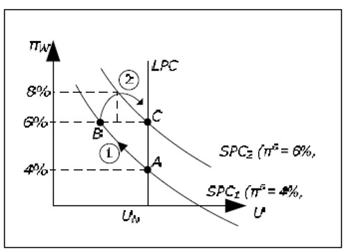
Fig. 15.3: From short run to long run.
- Point A: We start at point A which is on LPC where the economy is in equilibrium. Say that expected inflation is 4% so we are also on the SPC1 corresponding to an expected inflation of 4%. Since we are in equilibrium, inflation and the growth of the money supply is equal to wage inflation and these must be equal to expected inflation. In point A we therefore have π = πM = πw = πe = 4%.
- Movement 1: Suppose that πM suddenly and unexpectedly rises to 6%. The AD curve will then glide upward faster than the AS curve and Y will increase and π will increase. When Y increases, L increases and U will fall. Since the increase is not expected, inflation expectations will not change and neither will SPC. We move up along SPC 1 and πW increases. According to the discussion in section X, π and πW will eventually increase until they reach 6% and we move up to point B. So far, the discussion is completely consistent with the Keynesian model (as we have not replaced the SPC).
- SPC1 SPC2: As inflation is 6% at point B, inflation expectations must eventually increase. If inflation was 4% for a long time and it rises to and stabilizes at 6%, it is reasonable to expect future inflation to be 6%. In the synthesis, SPC shifts upwards to SPC2 which applies to πe = 6%.
- Point B: When inflation expectations have become 6%, we are below the new short-run Phillips curve. When the economy is at point B with unemployment below the natural rate, wages will rise by more than 6%. From SPC2 we can conclude that a wage inflation of 8% is consistent with an expected inflation of 6% when unemployment is equal to UB.
- Movement 2: If wages, and therefore prices, rises by more than 6%, the AS curve will glide upwards faster than the AD curve which means that Y will fall and U will increase. This must continue until we reach point C, where we once again are in equilibrium.
Note that in the Keynesian model SPC1 is the only Phillips curve and it is valid in the long run as well. In this model, there is no “movement 2”. The economy may remain in point B with π = πw = πM = 6% if this is desired by the government. The economy may return to point A by using restrictive fiscal and monetary policy.
In this section, inflation expectations did not change until we reached point B. This choice was more of a pedagogical choice to isolate and study each event individually. In reality, it is more likely that inflation expectations will slowly increase as we begin to move from point A to point B as inflation increases in this move. We would then have a movement from A to C more similar to movement 3 in the figure below. If the change in πM was announced prior to the actual change, it is possible that πe immediately changed to 6% at point A. We would then see the movement 4 directly from A to C (which, however, may take some time because of wage contracts).
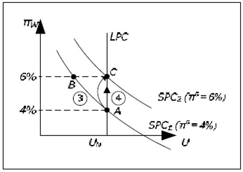
Fig. 15.4: From short to long run with a faster change in inflation expectations.
NAIRU
From the neo-classical synthesis, another important conclusion may be drawn. In order to keep U below UN, you need an accelerating inflation. Suppose that full employment is compatible with 4% inflation in the long run. In the Keynesian model, we can keep U below UN if we accept that inflation is above 4%. An inflation of, for example 7%, would keep the U below UN indefinitely. In the neoclassical synthesis, this will not work. If we want to keep U below UN, we must accept an ever higher inflation. In order to keep U one percentage unit below UN we might need an inflation of 7% in the first period, 9% in the second period, then 13% and so on.
Figure 15.3 will explain why. In order to reduce unemployment below UN, the growth rate in money supply must increase (unexpectedly). If nothing else is done, U will fall back to UN (now with a higher inflation). In order to keep U below UN, πM must increase again and again at an accelerating rate. Only the natural rate of unemployment, UN, is compatible with a non-accelerating inflation and this rate is therefore often called the NAIRU (Non-Accelerating Inflation Rate of Unemployment).
SAS-LAS-AD model of the neo-classical synthesis
AS-AD in the Keynesian and the classical model
First, a brief review of the AS-AD model according to the classical and the Keynesian model when W is constant and exogenous.
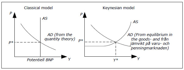
Fig. 15.5: The two AS-AD models.
According to the classical model, aggregate supply is independent of the price level and equal to potential GDP. Potential GDP is the amount produced when U = UN and the AS curve becomes a horizontal line through YPOT.
The AD curve in the classical model consists of combinations of Y and P where the quantity theory M·V = P· Y is satisfied. Aggregate demand is equal to the aggregate supply according to Say's Law. In the classical model, one starts from Y and finds P from the AD curve. The only function of the AD curve in the classical model is to determine the price level.
The AD curve slopes downwards in the Keynesian model as it does in the classical model but interpretation and the reason are quite different. In the Keynesian model, you start with P and you find YD from the AD curve. Here, the AD curve slopes downwards because when P falls,R decreases, I increases and YD increases (see section Aggregate demand). Another difference is that the AD curve may be affected by fiscal and monetary policy in the Keynesian model but not in the classical model.
In the Keynesian model, the AS curve is horizontal for low value of Y. In this region, the AS curve determines P while the AD curve determines GDP. Aggregate supply will be equal to aggregate demanded by the reverse Say's Law. For higher values of Y you need higher prices to stimulate aggregate and the AS curve will slope upwards. In this region, the AS and the AD curves simultaneously determine P and Y.
SAS, LAS, and AD
In the neo-classical synthesis, the Keynesian model is correct in the short run while (a slightly modified version of) the classical model applies in the long run. We therefore need to reconcile the AS-AD analysis of these models. In synthesis, the following concepts are introduced:
- Long-run aggregate supply (LAS): The classical AS curve (L for Long run)
- Short-run aggregate supply (SAS): The Keynesian AS curve (S for Short run)
In synthesis, it is the Keynesian AD curve that must be used. We can combine SAS, LAS, and AD in the same graph.
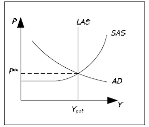
Fig. 15.6: SAS, LAS, and AD.
We begin by drawing them in such a way that both models agree in the determination of Y, Y = YPOT. In the synthesis, this corresponds to long run equilibrium – there is no tendency for Y to increase or decrease.
Note that the price level is determined in according to the Keynesian model both in the short and the long run (as we use the Keynesian AD curve). There is no reason however, to believe that this price level is consistent with the quantity theory. In other words, the classical AD curve (not shown) may intersect LAS at a completely different P. The quantity theory in levels need not hold in the neoclassical synthesis neither in the short run nor in the long run. However, the quantity theory in rates (π = πM) must hold in the long run. Therefore, it is not entirely correct to claim neo-classical synthesis reduces to the classical model in the long.
The dynamics from the short to the long run
We will now describe the dynamics from short to the long run in the LAS-SAS-AD model. To avoid having AS and AD curves “gliding”, we will assume that π M = 0. The case πM ≠ 0 is not much harder to analyze.
We begin by analyzing an increase in MS (πM is still zero – except for the brief when MS increases, which we assume is very short). We start in the long-run equilibrium as in Figure 15.6. Initially π = πw = πe = 0.
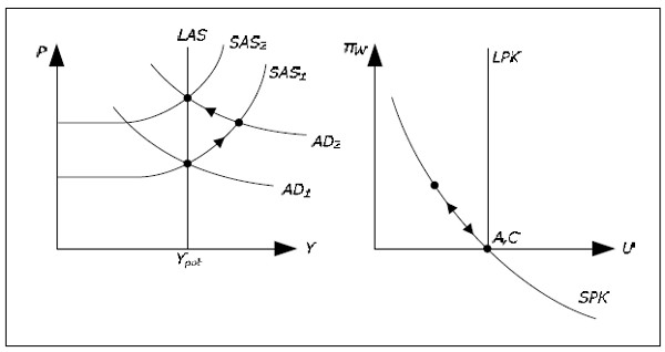
Fig. 15.7: Dynamics in the neo-classical synthesis.
- We are in the initial point A.
- When MS increases, the AD curve moves outwards from AD1 to AD2.
- We move from point A to point B. Y increases and P increases.
- As Y increases, U falls and we moving to point B on the SPK.
- At point B on the SPK, wages increases.
- When wages increase, the SAS curve will shift upwards.
- When the SAS curve shifts upwards, Y will fall and U will again increase. We ove back along the SPK.
- The SAS curve must continue to shift upwards as long as Y > YPOT. It will shift from SAS1 to SAS2 and we move to point C. We are back on the LAS and we are back on the LPK.
Whenever you use the neo-classical synthesis for your analysis, you should begin as if you where using the Keynesian model (with exogenous wages). This will give you the short-run outcome. To obtain the long-run results, remove the assumption of exogenous wages. Let wages adjust so that you will return to LAS and LPC.