Growth theory
- Details
- Category: Macroeconomics
- Hits: 10,424
The purpose of this chapter is to try to explain the growth in GDP. The models in this chapter are very different from the rest of the models in this book as they use only the production function and factors of production to explain growth.
Growth models are important, for example, if you want to understand why some countries grow faster and have a higher living standard than other countries. By growth, we mean the percentage change in real GDP. We use real GDP to eliminate the effect of inflation. In this chapter, it is perfectly OK to think of inflation as being zero in which case real and nominal GDP bare the same.
In this chapter we begin by describing the aggregate production function. The rest of this chapter will look at some different growth theories.
The aggregate production function
Imagine the national economy during a short period of time (say one week). We denote:
- L: the total amount of work used during this period (by all individuals in the economy).
- K: the total amount of capital used.
- Y: the total amount of finished goods produced during this period (real).
It is still the case that L and Y are flows while K is a stock. During a short period of time, we can assume that the amount of capital is constant.
The aggregate production function, or simply the production function is a function that relates L, K and Y. Specifically, we assume that Y is a function of L and K :
Y = f (L , K)
In most cases, we will not specify exactly what the function f looks like. However, we always assume that f is increasing in L and K, that is, when we use more labor and/or more capital, we will produce more goods.
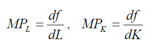
The marginal product of labor and capital
We define the marginal product of labor, MPL as the derivative of f with respect to the L – that is, as (approximately) how much Y will increase when L increases by one unit. We also define the marginal product of capital, MPK as the derivative of f with respect to K. Note that MPL and MPK will depend on both L and K ( MPL and MPK are functions, not variables).
- Since f is increasing in L, MPL must be positive for all values of L and K.
- MPL assumed to be decreasing in L – the more work that is used, the lower the marginal product of labor.
- MPL assumed to be increasing in K – the more capital, the higher the marginal product of labor
- In the same way, MPK must be positive for all values of L and K.
- MPK is assumed to be decreasing in K and increasing in L.
When we view Y as a function of L holding K fix, Y will be increasing in L but at a decreasing pace (due to the fact that MPL is positive but decreasing in L ).
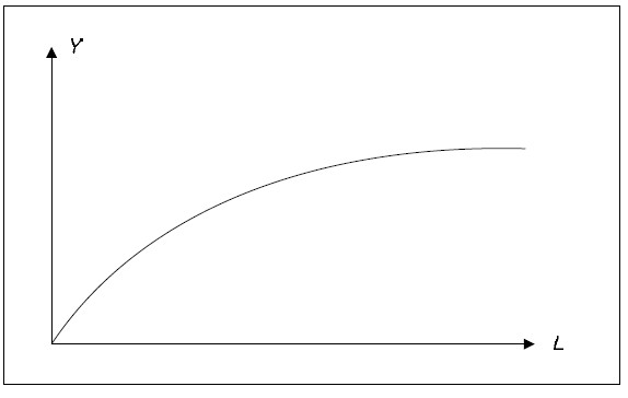
Fig. 9.1: Production function.
We define labor productivity as Y / L, that is, as GDP per hour worked. Labor productivity tells us how much we can produce using one hour of labor and it depends on the amount of capital as well as the technology.
Production function and Growth
From the simple production function Y = f (L, K), we can identify three sources of growth:
- An increase in L.
- An increase in K.
- A change in the function f
The first two represent the growth of the factors of production. L may increase if the population grows, if we have more individuals in the workforce, or if unemployment falls. K increases if investment are large as they are if total savings is large.
The function f need not be the same function over time. It is possible that Y increases even though L and K are fixed. When f changes so that the same amount of the factors of production will produce more output we say that we have technological progress or productivity growth. With technological progress, MPL and MPK will typically increase for given values of L and K, that is, the productivity of the factors increase.
Education and growth in human capital are important aspects of growth in GDP. Human capital is treated in different ways in the literature:
- You can think of human capital as being included in K – with this view education is a type of investment.
- You can add another variable in the production function: Y = f ( L, K, H ) where H is the amount of human capital and K amount of physical capital.
- The amount of human capital may affect the function f. The more human capital, the more can be produced from the same amount of L and K. With this view, increasing the amount of human capital will lead to productivity growth.
Growth Accounting is the activity in which we try to figure out how much of the growth in GDP is due to growth in L, growth in K and growth in productivity.
Growth Theories
The classical growth theory
The production function will not provide us with a theory or explanation of growth. It is only a convenient tool that helps us breaking down growth into its components. However, there are many growth theories that try to go a step further. The oldest of these theories is the so-called classical growth theory which is primarily associated with Thomas Robert Malthus.
The classical growth theory should not be confused with the classical model that we will look at in the next chapter. Also, the classical growth theory, which was developed in the late 1700s, has little or no relevance today. We present it so that you can better understand more modern growth theories.
In short, the classical growth theory may be described as follows:
- Due to technological development, the amount of capital increases and the marginal product of labor rises.
- GDP per capita rises. With higher living standards, the population will increase.
- As population increases, labor productivity will fall (more individuals but the same amount of capital).
- GDP per capita will fall again. When GDP per capita has fallen to a level just high enough to keep the population from starving, the increase in population will cease.
Destruction of capital, for example, through a war, works in the opposite way. The marginal product of labor falls, GDP per capita falls and the population decreases. This will again lead to an increase in the marginal product of labor and GDP per capita return to the "survival rate".
The main point of the model is that population growth will always eliminate the positive effects of technological development and GDP per capita will always return to the survival level. This very "dismal" growth theory was prominent in the early 1800s, and economics to this day is sometimes called the "dismal science".
Today we know that the predictions of the model where incorrect. During the rest of the 1800s Europe experienced a growth in GDP per capita. Although the population growth was high, it was not nearly sufficient to eliminate the positive effects of technological development.
The neoclassical growth model
The main purpose of another important growth model, the neoclassical growth model, is to explain how it is possible to have a permanent-growth in GDP per capita. The model was developed by Robert Solow in the 1960s and it is sometimes called the Solow growth model or the exogenous growth model.
The neoclassical growth model should not be confused with the neoclassical synthesis, which we will study in chapter 10. "Neo" means "new" – the neoclassical growth theory is a “new version” of the classical growth model.
The crucial difference between the classical and neoclassical growth models is that the population is endogenous in the former and exogenous in the latter. In the classical model, the population will increase or decrease depending on whether GDP per capita is higher than or lower than the survival level. In the neo-classical model population growth is not affected by GDP per capita (however, the population growth will affect the growth in GDP per capita).
In the neo-classical model, it is the technological progress only that affects the GDP per capita in the long run. We will have a permanent increase in GDP per capita when there is a technological development that increases the productivity of labor. Permanent growth in GDP then requires continuous technological progress.
It is not possible for the government, except temporarily, to affect the growth rate in the neoclassical growth model. The government might be able to affect GDP per capita (and this is the growth rate) but the growth rate always returns to the level determined by the technological progress. The same is true for savings. An increase in savings may have a temporary effect on GDP but it will have no effect in the long run.
Endogenous growth theory
Endogenous growth theory or new growth theory was developed in the 1980s by Paul Romer and others. In the neo-classical model, technological progress is an exogenous variable. The neoclassical growth model makes no attempt to explain how, when, and why technological progress takes place.
The main objective of the endogenous growth theory is to make the technological progress an endogenous variable to be explained within the model, hence the name endogenous growth theory.
There are many different explanations for technological progress. Most of them, however, have a lot of common characteristics:
- They are based on a constant return to scale for capital. Thus, MPK is not a decreasing function of K in these models.
- They consider technological development as a public good.
- They focus more on human capital.
- It is possible for the government to affect the growth rate. Higher savings also leads to higher growth, not just higher GDP per capita.
- They predict the convergence of GDP per capita between countries in the long run. This is a consequence of the public good property of technological developments.
Separation of growth and fluctuation
It is often useful to separate the evolution of a variable that grows over time into a trend and fluctuations around the trend. The graphs below show such a separation for real GDP.
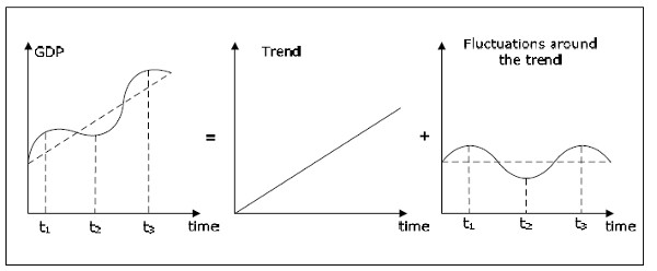
Fig. 9.2: Growth and the fluctuation around the trend.
The left diagram shows a stylized graph of real GDP over time. It demonstrates the two important characteristics of real GDP. GDP fluctuates over time and GDP grows overtime – at least over a longer period of time. The left graph is the sum of the middle graph and the right graph. The middle graph shows the trend in GDP. The trend represents the second characteristic of GDP – the fact that GDP grows over time. The right graph shows the fluctuations around the trend (cycles) of GDP. These fluctuations around the trend represent the first property of GDP.
In macroeconomics it is common to study trends and cycles separately. The purpose of growth theory is to investigate the trend while most of the macroeconomics apart from growth theory is about the cycles. The trend is about the very long-run perspective of the economy while cycles are about the short and medium run. The rest of this is all about cycles and not at all about trends. Therefore, when you think of GDP in the remaining chapters, you should think of GDP as in the right-hand graph: GDP has cycles but no trend. Basically, we will study GDP where the trend has been removed.